6 Parameter Estimation: Advanced Techniques

In Chapter 4, we introduced the basics of parameter estimation using maximum likelihood and the Nelder–Mead algorithm as a general-purpose optimization method. To recap, we can think of Nelder–Mead as a triangle (when we estimate two parameters) that tumbles down the negative log-likelihood surface until it comes to rest in the valley of a (hopefully global) minimum. While this approach is intuitive and accessible, we have also discussed its limitations in several important ways.

In this chapter, we introduce more advanced techniques for both optimization and parameter inference. These methods are designed to address key challenges encountered in earlier sections: avoiding local minima and modeling multiple participants in hierarchical data structures.

For the purpose of parameter estimation, we will introduce Differential Evolution (DE), which offers more robust search strategies (in comparison to Nelder-Mead). DE is a population-based, gradient-free algorithm. Instead of exploring the cost function with a single point, DE maintains an entire population of parameter vectors distributed across the space. The population is iteratively updated, allowing DE to be especially effective in tackling complex, multimodal optimization problems.

When fitting a DDM, we are often interested not only in the best-fitting parameter values, but also in the uncertainty associated with those estimates. For instance, suppose we estimate a peak latency of \(\tau = 0.12\) seconds from a DMC fit. This value is only a point estimate, and repeating the experiment would yield different data due to sampling variability, most likely resulting in a different estimation of \(\tau\). To meaningfully interpret this estimate, for example, when comparing it to values from another study, we must ask: How much can we trust this value? Is \(\tau = 0.12\) tightly constrained by the data, or is a wide range of \(\tau\) values nearly as plausible?

Bayesian inference provides a principled framework for answering such questions.³⁷ In the Bayesian approach, we aim to estimate the full posterior distribution over parameters, which captures both point estimates and associated uncertainty. Additionally, we can incorporate prior knowledge to constrain or regularize estimation, and naturally extend the framework to account for hierarchical data structures.

To this end, we will introduce Markov Chain Monte Carlo (MCMC) methods, including, Differential Evolution MCMC (DE-MCMC), which combines the strengths of population-based global search with the formal machinery of Bayesian inference. In short, this chapter will extend your modeling toolkit with methods that are more powerful, more flexible, and often better suited for real-world data analysis, especially when dealing with individual differences, complex models, or the need to quantify uncertainty.

6.1 Advanced Algorithms for Optimization

6.1.1 Differential Evolution

Differential Evolution (DE) is a population-based optimization algorithm introduced by Storn and Price (1997). The algorithm begins by generating a set of \(NP\) random parameter combinations, typically sampled uniformly across the parameter space. These combinations, called population members, form the initial generation.³⁸ At each iteration, DE creates a new generation by recombining and mutating existing members. Because of this biological metaphor, DE is sometimes referred to as a genetic algorithm, and its iterations are described in terms of “generations,” “mutation,” “children,” and so on.

A common strategy to update the population is as follows: For each current parameter vector \(\theta_{i,g}\) in generation \(g\) (where \(i \in \{1, ..., NP\}\)), the algorithm selects three distinct other members from the population: \(x_{r0,g}\), \(x_{r1,g}\), and \(x_{r2,g}\). It then adds a scaled difference between two of them to the third, forming a proposal vector (a “mutation”) \(\theta^*_{i}\)

\[\begin{equation} \tag{6.1} \theta^*_{i} = x_{r0,g} + F \cdot (x_{r1,g} - x_{r2,g})\,. \end{equation}\]

This proposal is then evaluated with respect to the cost function (e.g., the negative log-likelihood). If the proposal yields a better fit than the current member \(\theta_{i,g}\), it replaces it in the next generation. This process is repeated for all members of the current generation \(g\), producing a new generation \(g + 1\). The factor \(F\) controls the mutation’s scale and is typically set to a value around 0.8 (it must lie between 0 and 2).

Figure 6.1 illustrates the basic idea using the same negative log-likelihood surface introduced in Section 4.2.1. Unlike the earlier 3D plot, we now show a 2D contour representation, which makes it easier to visualize how the population evolves. The black circles represent the current population members, each labeled with a number. The blue point marks a selected target member \(\theta_{1,g}\), which will undergo mutation (as described in Equation (6.1)).

Two proposed mutations for the first member are shown, one successful, the other not:

• In the first case, the algorithm randomly selects \(x_{19,g}\), \(x_{3,g}\), and \(x_{9,g}\), highlighted in green. It computes the difference between members 3 and 9 (the green dotted arrow), scales it, and adds it to member 19 (solid green arrow).³⁹ The result is the proposed mutation \(\theta^*_{1}\), shown as an orange dot labeled “1*”. Since this proposal yields a lower negative log-likelihood than the original, it is accepted, and \(\theta_{1,g}\) is replaced by \(\theta^*_{1}\) in the next generation \(g+1\). In the language of genetic algorithms, we might say that the “child” has higher fitness than its “parent.”

• In the second case, the algorithm selects \(x_{14,g}\), \(x_{8,g}\), and \(x_{5,g}\), highlighted in red. The mutation proceeds in the same way, but this time the resulting proposal has a higher negative log-likelihood. As a result, the proposal is rejected, and \(\theta_{1,g}\) remains unchanged for the next generation \(g+1\).

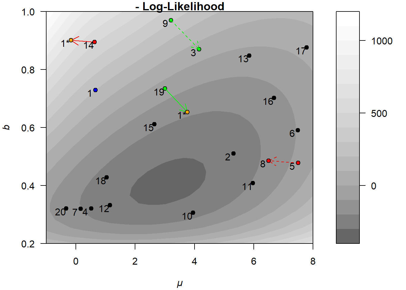
Figure 6.1: Illustration of a mutation in the DE algorithm.

Although DE is a powerful global optimization method, its basic structure is surprisingly simple and can be implemented in just a few lines of R code. The following function provides a minimal, but still functional implementation of the core DE loop:

# fn => the function to optimize
# init_lower, init_upper => the space for initiating the population
# pop_size => the size of the population
# F_val => the scaling factor when taking the difference
# max_iter => the maximum number of iterations
my_de <- function(fn, init_lower, init_upper, F_val = 0.8, max_iter = 200) {
  D <- length(init_lower) # number of parameters
  pop_size <- 10 * D # number of population members (10 * D is often recommended)

  # initiate the first population
  pop0 <- replicate(pop_size, runif(D, init_lower, init_upper))
  costs0 <- apply(pop0, 2, fn) # evaluate initial population
  idxs <- seq_len(pop_size)

  # initiate a container to store all the populations and cost values
  all_pops <- list(pop0)
  all_costs <- list(costs0)

  for (iter in 1:max_iter) {
    pop <- all_pops[[iter]] # copy the previous generation/population...
    costs <- all_costs[[iter]]
    # and then update each member
    for (i in idxs) {
      # Choose 3 distinct members different from i
      idxs_i <- idxs[-i]
      r123 <- sample(idxs_i, 3)
      x0 <- pop[, r123[1]]
      x1 <- pop[, r123[2]]
      x2 <- pop[, r123[3]]

      # Mutation: proposal vector = x0 + F * (x1 - x2)
      proposal <- x0 + F_val * (x1 - x2)

      # Test for acceptance
      fp <- fn(proposal)
      if (fp < costs[i]) {
        pop[, i] <- proposal
        costs[i] <- fp
      }
    }
    # Finally: Store the update generation
    all_pops <- c(all_pops, list(pop))
    all_costs <- c(all_costs, list(costs))
  }

  # Return best solution and all generations
  best_idx <- which.min(costs)
  list(
    par = pop[, best_idx], value = costs[best_idx], n_iter = length(all_pops), 
    all_pops = all_pops, all_values = all_costs
  )
}

Because DE explores the parameter space using an entire population, it is particularly robust to local minima and effective in navigating wide and complex cost functions. This makes it especially well suited for fitting DDMs, where the likelihood surface often exhibits many peaks and valleys once we move beyond two parameters.

6.1.1.1 Demonstration

To illustrate the robustness of DE, we consider the Rastrigin function, a mathematical function explicitly designed to challenge optimization algorithms by introducing a large number of local minima.

rastrigin <- function(prms) {
  x <- prms[1]
  y <- prms[2]
  20 + x^2 + y^2 - 10 * (cos(2 * pi * x) + cos(2 * pi * y))
}

From the following 3D visualization, it is easy to see why this function is difficult to optimize: it contains many local minima that can trap algorithms into suboptimal solutions.

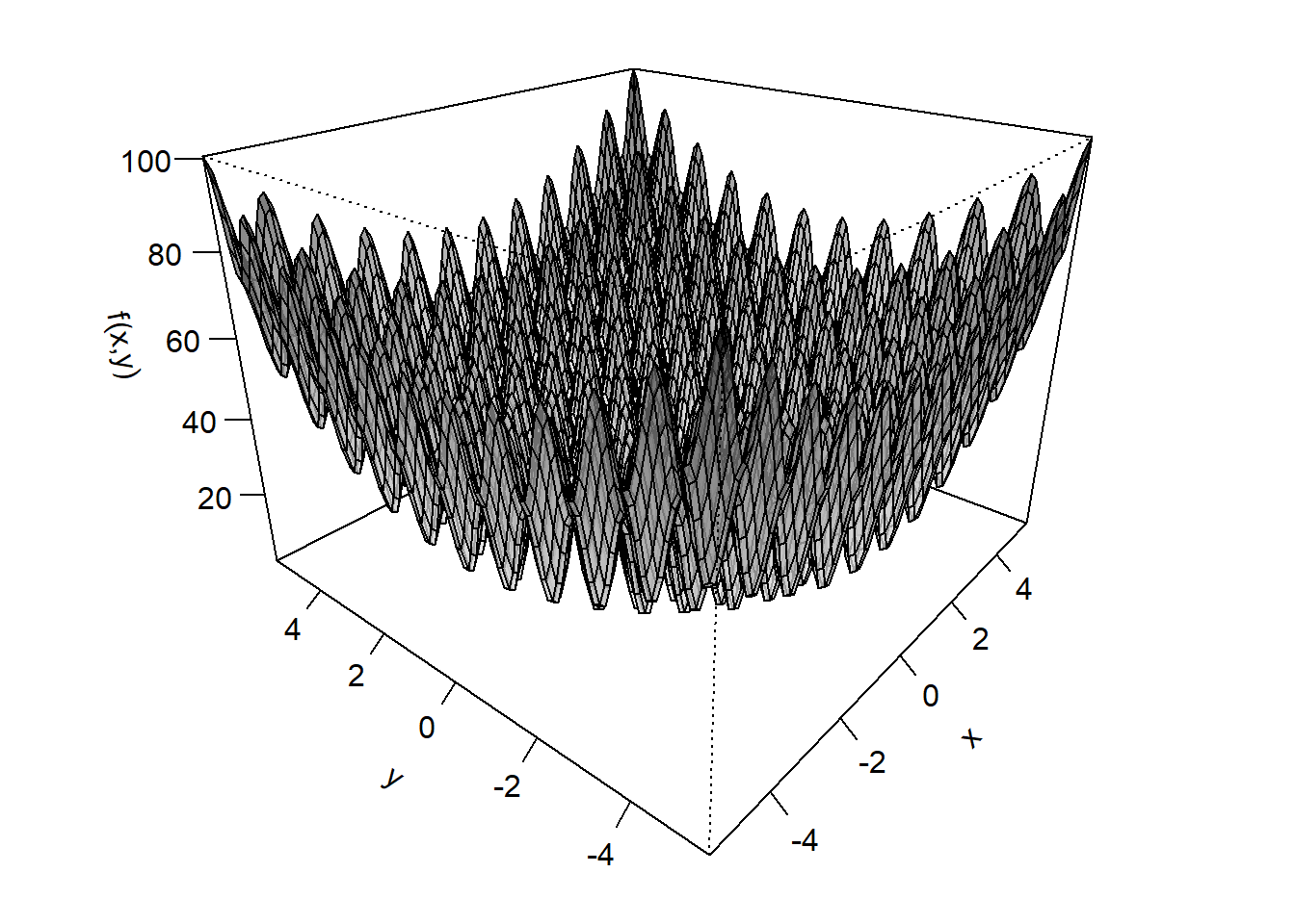
Figure 6.2: Visualization of the Rastrigin function.

Although this function looks like a beast, it actually has a well-defined global minimum right at the center at \(x = 0\) and \(y = 0\)! Let us now test whether our my_de() implementation can handle the challenge and find this minimum.

set.seed(2) # because the initial population is drawn randomly
out <- my_de(fn = rastrigin, 
             init_lower = c(-4, -4),
             init_upper = c(4, 4))
out$par

## [1] -6.713012e-11  2.762669e-09

out$value

## [1] 0

Apparently it can! Now let us make the problem more difficult by initializing the population farther away from the global minimum:

set.seed(2) # because the initial population is drawn randomly
out <- my_de(fn = rastrigin, 
             init_lower = c(-5.5, -5.5),
             init_upper = c(-1, -1))
out$par

## [1] -2.424665e-09  1.525275e-09

out$value

## [1] 0

Even in this case, our DE implementation successfully finds the global minimum. To observe DE in action, we plot several intermediate populations from the previous run in Figure 6.3. For this, we use a 2D projection of the Rastrigin function, which makes it easier to compare how the population (shown in blue) evolves across generations. Within each generation, the parameter combination with the lowest cost function value is shown in orange.

Figure 6.3: Illustration of how DE searches the Rastrigin function for its global minimum. The population on iteration/generation 1, 10, 20, 30, 40, and 50 are shown in separate panels, as indicated by the respective number above each panel. Darker shadings indicate lower values of the Rastrigin function

From Figure 6.3, we can see that the entire population moves rapidly toward the global minimum within the first 30 generations (the upper four panels). After that, most population members cluster closely to the global minimum or in adjacent local minima (lower left panel). Finally, by generation 50, all members have contracted tightly and settled around the global minimum (lower right panel).

Let us finally compare DE’s performance to that of the Nelder–Mead algorithm using the nmkb() function from the dfoptim package:

nmkb(par = c(0.5, 0.5), 
     fn = rastrigin, 
     lower = c(-4, -4),
     upper = c(4, 4))

## $par
## [1] 2.984883 2.984835
## 
## $value
## [1] 17.9092
## 
## $feval
## [1] 68
## 
## $restarts
## [1] 0
## 
## $convergence
## [1] 0
## 
## $message
## [1] "Successful convergence"

Apparently, Nelder-Mead struggles to find the minimum. In fact, even though we have placed the starting point near the global minumum, nmkb() failed to find it and actually ended up worse than initially placed. Figure 6.4 traces the search line of the Nelder-Mead run with the starting point shown in blue and the point of convergence in orange. We can easily see that Nelder–Mead did not explore the surface very thoroughly. Instead, it tumbled away from the global minimum and ended in a far away local minimum!

Figure 6.4: Illustration of how the Nelder-Mead algorithm searches the Rastrigin function for its global minimum.

6.1.1.2 Additional Comments

In the previous section, we saw that DE is a powerful algorithm for avoiding local minima. For completeness, however, we want to mention that many DE implementations offer additional tuning options that can improve performance and adapt the algorithm’s behavior.

One common extension is crossover. During crossover, the mutation vector \(\theta_i^*\) is not used as-is, but instead combined with the original parameter vector \(\theta_{i,g}\) to form a trial vector \(\omega_i^*\). Typically, this is done by randomly selecting a subset of parameters from the proposal \(\theta_i^*\), while the remaining parameters are taken from the current solution \(\theta_{i,g}\). This process is controlled by the crossover probability \(CR\): the higher the value of \(CR\), the more elements from \(\theta_i^*\) are used. The resulting vector \(\omega_i^*\) is then used to evaluate whether the “child” replaces its “parent” in the population. Crossover introduces additional variability and can help balance exploration and exploitation of the parameter space.

Another practical consideration is the use of box constraints, which limit the allowed range of each parameter. We are already familiar with this concept from Nelder–Mead, and many DE implementations provide similar boundary arguments.

Importantly, DE is not a single fixed algorithm, but rather a flexible family of strategies that differ in how they generate new population members. These strategies are often described using shorthand labels like "DE/rand/1/bin" or "DE/local-to-best/1/bin" (Price, Storn, and Lampinen 2006). Each part of the name specifies:

• Which population members are used for mutation,
• How many difference vectors are involved, and
• What kind of crossover is applied.

For example, "DE/rand/1" is the strategy used in our my_de() implementation: three randomly chosen individuals generate a mutation vector, and no crossover is applied. In contrast, "DE/local-to-best/1/bin" incorporates the current best-known parameter combination (local-to-best) to speed up convergence and applies binomial (bin) crossover. During binomial crossover, each element of \(\theta_i^*\) is considered separately, with a fixed chance of being swapped into the trial vector \(\omega_i^*\). This is in contrast to exponential crossover, which replaces a contiguous block of parameters.

From our perspective, one does not need to worry too much about choosing a specific DE strategy or tuning the crossover rate \(CR\): the default settings in most software packages already work well in many cases.⁴⁰ In R, the package DEoptim provides a flexible DE implementation via the function DEoptim(). This is also the function used internally by dRiftDM (and also by DMCfun), and serves as the default optimization algorithm in dRiftDM.

To summarize, DE is a robust and powerful algorithm that is particularly good at escaping local minima. However, its downside is that it is computationally expensive: for each generation, the model must be evaluated for every member of the population. As a result, DE typically requires many more function evaluations than simpler downhill algorithms like Nelder–Mead. However, the additional computational cost comes with the benefit of increased reliability, as it typically does not need require an initial grid search or repeated runs, such as Nelder-Mead with different starting values.

DE has had a significant influence on numerical optimization due to its robustness and ease of implementation. As we will see in the next section, it even serves as the foundation for a powerful Bayesian sampling algorithm: Differential Evolution MCMC (DE-MCMC).

6.1.2 Exercise: Simplex vs. Differential Evolution

Let us now use the knowledge about Nelder Mead and DE algorithm and run a parameter recovery study. To do so, we simulate synthetic data under known parameters and then fit the model to the data in an attempt to recover those original values.

1.) Create the SSP model using dRiftDM without any trial-by-trial variabilities. Then simulate 50 data sets with 100 trials per congruency condition using the function simulate_data(). Use the following parameter ranges (adapted from White, Servant, and Logan 2018):

• b: 0.35 – 0.95
  
• non_dec: 0.20 – 0.45
  
• p: 2.0 – 5.5
  
• sd_0: 1.0 – 2.6

2.) Fit the SSP model to each of the 50 data sets twice:

• Once using Nelder–Mead, and then
• using Differential Evolution.

To speed up computation, increase the step sizes in the model’s discretization settings (i.e., dt, dx).

3.) Compare the estimated parameters to the original parameters using scatterplots, separately for each optimization approach. What do you observe? Did you expect this? What does this tell you about SSP?

6.2 Bayesian Inference

Bayesian inference offers a different perspective on parameter estimation than classical MLE. Instead of focusing solely on finding the best-fitting parameter values, Bayesian methods aim to describe the entire distribution of plausible parameter values, given the observed data and prior knowledge.

The core of Bayesian inference is Bayes’ rule, a fundamental equation for inverting conditional probabilities. In the context of DDMs, we’ve already encountered the conditional probability \(p(y | \theta)\), which describes the probability of observing RTs \(y\) given a set of parameters \(\theta\). When we assume \(y\) to be fixed, we can examine how this probability changes as a function of \(\theta\). This leads to the likelihood function, \(\mathcal{L}(\theta | y)\).

As discussed earlier in Section 4.1.2, \(L(\theta | y)\) is not the same as the probability density of \(\theta\) given \(y\) (i.e., \(p(\theta|y)\)). One reason is that \(\mathcal{L}(\theta | y)\) does not integrate to 1. However, Bayes’ rule allows us to derive this conditional probability, which is generally called the posterior distribution

\[ p(\theta | y) = \frac{p(y | \theta) \, p(\theta)}{p(y)}\,, \] where

• \(p(\theta | y)\) is the posterior distribution, describing the probability of the parameter vector \(\theta\) after observing data \(y\),
• \(p(y | \theta)\) is the likelihood, expressing how well the model with parameters \(\theta\) explains the data \(y\). This might be a bit confusing, as we previously termed \(\mathcal{L}(\theta|y)\) to be the likelihood. However, both quantities are essentially the same, it’s just a matter of what we are interested in. In Bayes’ rule we ask for the probability of the data given the parameter,
• \(p(\theta)\) is the prior distribution, representing our beliefs about the parameters before observing the data,
• and \(p(y)\) is the marginal likelihood (or evidence), which normalizes the posterior and ensures it integrates to 1. Although we will not focus on this term in the present chapter, the marginal likelihood is an important ingredient for Bayesian model comparison.

In short, Bayesian inference provides a framework for estimating the posterior distribution \(p(\theta | y)\) for parameters such as the drift rate \(\mu\), boundary separation \(b\), or non-decision time \(t0\). Because the posterior is a full distribution rather than a point estimate, we can straightforward quantify uncertainty in a principled way. Moreover, because the posterior is shaped by both the likelihood and the prior, we can incorporate domain knowledge directly into the estimation process.

6.2.1 Bayes’ Rule and Bayesian Sampling

An issue in the application of Bayes’ rule is that the required mathematics for obtaining the posterior distribution is often quite complex. In order for it to be derived analytically, we have to know how to multiply the likelihood with the prior. Additionally, to compute the denominator, \(p(y)\), we have to integrate over all possible values of \(\theta\), that is,

\[ p(y) = \int p(y | \theta) \, p(\theta) \, d\theta \,. \]

Thus, in many cases, deriving the posterior distribution is either very tedious or simply impossible, especially for complex models like the DDM. Fortunately, there are two “tricks” that we can use to reduce the complexity while keeping the core idea of Bayesian inference untouched.

First, when assuming the observed data to be fixed, the marginal probability \(p(y)\) is a constant that merely ensures the posterior integrates to 1. However, since it does not affect the shape of the posterior, we can drop it for simplicity, and say that the posterior is proportional to the product of the likelihood and the prior,

\[ p(\theta | y) \propto p(y | \theta) \, p(\theta)\,, \] and we call the posterior unnormalized in this case.

Second, instead of doing the mathematics by hand, we can delegate the task of exploring the posterior to the computer using sampling-based methods. Specifically, while we may not know the shape of \(p(\theta | y)\) in closed form, we can evaluate all the components on the right-hand side of Bayes’ rule. This allows us to write an algorithm that plugs in different values of \(\theta\) into the likelihood and prior, calculates their product, and gains insight into how the posterior behaves as a function of \(\theta\).

Exploring the unknown posterior distribution is conceptually very similar to how we optimized the unknown negative log-likelihood earlier. However, Bayesian sampling methods behave differently. In optimization-based approaches (such as maximum likelihood), the goal is to find a single best-fitting set of parameters. That is, the values that minimize (or maximize) an unknown cost function. Remember, for example, how Nelder–Mead placed a triangle on a surface that tumbled down the hill until it reached a valley.

In contrast, Bayesian sampling methods do not aim to find just one optimal parameter set. Instead, they aim to characterize the posterior distribution. To do this, these algorithms are explicitly designed to operate stochastically rather than deterministically. When estimating \(\theta\), the algorithm moves toward areas of high posterior probability. But crucially, it does not stop once it arrives. Instead, it continues exploring the area, storing each visited \(\theta\) value as a sample from the posterior.

The longer we run the algorithm, the more the collected samples form an equilibrium distribution that matches the posterior.⁴¹ Thus, Bayesian sampling methods provide rich information about the posterior’s shape around its maximum. Most of the time, Bayesians use a class of algorithms called Markov Chain Monte Carlo (MCMC):

• Markov Chain, because each new proposal \(\theta^*\) depends only on the current state \(\theta^{(t)}\).
• Monte Carlo, because we use random sampling (rather than deterministic optimization) to explore the distribution.

6.2.2 Visualizing the Posterior

Let us visualize a posterior distribution and show how it differs from the likelihood function. In the following, we again consider the Ratcliff DDM as a function of the drift rate \(\mu\) and the decision boundary \(b\), based on the same exemplary data already used in Section 4.2.1 and Section 6.1.1.

The upper panel of Figure 6.5 shows the contour of the likelihood function \(p(y|\theta)\) (Note that this is not the log-likelihood function!). Here, we can already see why the logarithm of the likelihood is almost always used instead. The values range from zero to \(4 \cdot 10^{147}\), which distorts the color coding on the right side of the plot and results in less smooth contour lines compared to earlier visualizations. Nevertheless, the likelihood function resembles the previous contours of the log-likelihood (see, e.g., Section 6.1.1), with the most likely parameters located somewhere around \(\mu = 3.5\) and \(b = 0.4\).

To calculate the posterior \(p(\theta | y)\), we are forced by Bayes’ rule to specify a (joint) prior distribution for \(\mu\) and \(b\), \(p(\theta) = p(\mu,b)\). In the present example, we chose⁴²

\[ \begin{pmatrix} \mu \\ b \end{pmatrix} \sim N_2\left( \eta, \; \Sigma \right) \quad \text{with} \quad \eta = \begin{pmatrix} 6 \\ 0.6 \end{pmatrix} \quad \text{and} \quad \Sigma = \begin{pmatrix} 0.25^2 & 0 \\ 0 & 0.025^2 \end{pmatrix}\,. \]

This corresponds to assuming that \(\mu\) and \(b\) are independently distributed with separate normal distributions⁴³, that is,

\[\begin{align*} \mu &\sim N(6, \; 0.25^2) \\ \text{and }b &\sim N(0.6, \; 0.025^2) \,. \end{align*}\]

The joint prior is then simply the product of the individual prior distributions:

\[ p(\theta) = p(\mu, b) = p(\mu) \cdot p(b) \,. \] The middle panel of Figure 6.5 shows a contour plot of this (joint) prior distribution. Note that the prior settings are very very narrow here. For example, we assume that \(\mu\) lies between \(5.25\) and \(6.75\) with a probability of about \(99\%\). Normally, we would not have such strong beliefs about \(\mu\) and \(b\), especially because priors are specified before observing the data (not afterward, as in this educational example). However, these narrow priors are useful for demonstrating how the likelihood is combined with the prior to form the (unnormalized) posterior distribution, which is shown in the lower panel of Figure 6.5.

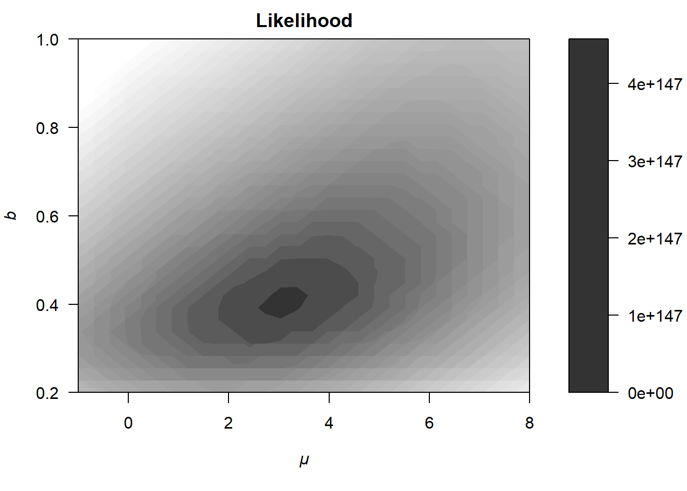
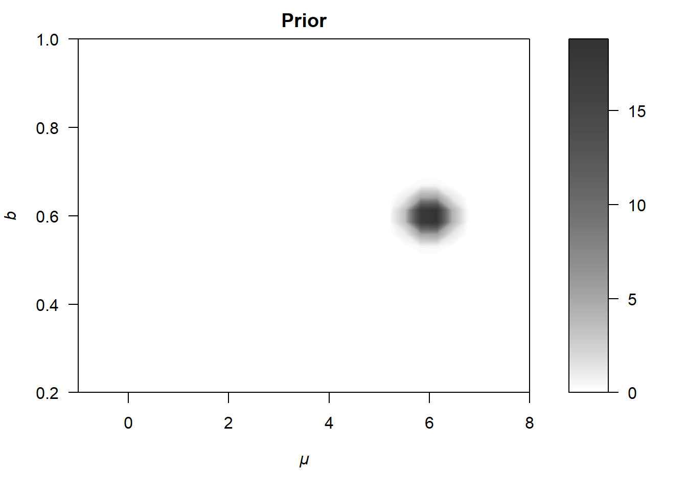
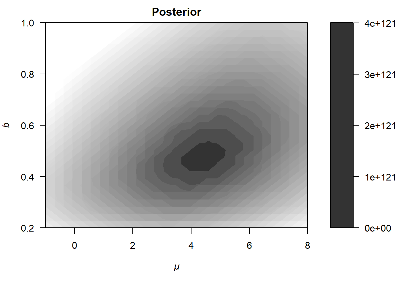
Figure 6.5: Illustration of how a likelihood (upper panel) differs from the posterior distribution (lower panel).

As is evident from the lower panel of Figure 6.5, the posterior is shifted slightly upward and to the right relative to the likelihood, such that the most probable parameters are now approximately \(\mu = 4.5\) and \(b = 0.5\).

6.2.3 Basics on MCMC

We can run an MCMC algorithm to explore the posterior distribution and gain rich information about the probability of parameters. In this section, we introduce a very simple, yet powerful algorithm that was one of the earliest of its kind: the Metropolis algorithm. The general procedure of this algorithm is as follows:

1. Start from an initial guess \(\theta_0\).
   
2. Propose a new value \(\theta^*\) by adding a random value drawn from a symmetric jumping distribution, for example, a (multivariate) normal distribution.
   
3. Compute the ratio \(r = \frac{p(\theta^*| y)}{p(\theta_i | y)}\), where \(i\) denotes the current iteration and \(p(\theta | y)\) refers to the posterior distribution (also known as the target distribution).
   
4. Accept or reject the proposal with probability \(\min(1, r)\).
   
5. Repeat from step 2 until a sufficient number of samples has been drawn.

Let us implement this algorithm for our example:

# create the model for our example
my_model <- ratcliff_dm(
  t_max = 1.5, dt = 0.01, dx = 0.01,
  obs_data = dRiftDM::ratcliff_synth_data
)

# create a function to easily calculate the posterior value
# prms => contains values for mu and b
calc_posterior <- function(prms) {
  
  # extract parameters
  mu <- prms[1]
  b <- prms[2]

  # calculate the likelihood value
  coef(my_model)[c("muc", "b")] <- prms
  likelihood <- exp(logLik(my_model))
  
  # evaluate the (joint) prior distribution 
  prior_val_mu <- dnorm(mu, mean = 6, sd = 0.25) # prior density
  prior_val_b <- dnorm(b, mean = 0.6, sd = 0.025) # prior density
  prior_val <- prior_val_mu * prior_val_b

  # posterior density = likelihood * joint prior
  posterior <- likelihood * prior_val
  return(posterior)
}

# create a function to perform Metropolis MCMC
# start_values => the initial set of parameters for mu and b
# n_samples => for how many iterations shall the algorithm run?
# sd_mu, sd_b => standard deviations of the normal distributions that are
# used to create theta_star
my_metropolis <- function(start_values = c(2, 0.3), n_samples = 1000,
                          sd_mu = 0.25, sd_b = 0.025) {
  # storages for our samples
  samples <- matrix(NA, nrow = n_samples, ncol = 2)
  posterior_vals <- numeric(n_samples)

  # starting values
  samples[1, ] <- start_values
  posterior_vals[1] <- calc_posterior(samples[1, ])

  for (i in 2:n_samples) {
    # get the parameter values from the previous iteration
    theta_prev <- samples[i - 1, ]
    posterior_prev <- posterior_vals[i - 1]

    # calculate a proposal by pertubating theta_prev
    rand_mu <- rnorm(1, mean = 0, sd = sd_mu) # draw a value to pertubate mu
    rand_b <- rnorm(1, mean = 0, sd = sd_b) # draw a value to pertubate b
    mu_star <- theta_prev[1] + rand_mu
    b_star <- theta_prev[2] + rand_b
    theta_star <- c(mu_star, b_star)

    # calculate the posterior (cac_posterior might crash for unreasonable values,
    # so put it into a tryCatch statement)
    posterior_star <- tryCatch(
      calc_posterior(theta_star),
      error = function(err) -Inf
    )

    # Compute acceptance probability
    accept_ratio <- posterior_star / posterior_prev
    r <- min(1, accept_ratio)

    # Accept or reject
    if (runif(1) < r) {
      samples[i, ] <- theta_star
      posterior_vals[i] <- posterior_star
    } else {
      samples[i, ] <- theta_prev # stay where you are
      posterior_vals[i] <- posterior_prev
    }
  }

  # return the samples
  colnames(samples) <- c("mu", "b")
  return(samples)
}

While this is quite a bit of code, most of it is actually concerned with extracting and setting parameter values. We start by creating the Ratcliff DDM with the exemplary data set. Then, we write a function calc_posterior() that calculates the value of the posterior distribution for a set of mu and b values (stored in prms). This is the function we visualized in the previous contour plot. Note that within calc_posterior(), we make use of the fact that the joint prior distribution can be obtained from the marginal distributions when assuming independence.

The largest part of the code snippet is dedicated to implementing our Metropolis MCMC algorithm my_metropolis(). In the beginning, we create containers and store the starting values (i.e., \(\theta_0\)). Then, we define a for loop, where a proposal \(\theta^*\) is generated by separately perturbing the parameter values in \(\theta_i\). The standard deviations of the normal distributions used for this perturbation are provided as arguments to the function and are chosen somewhat arbitrarily in this example. However, they play an important role in controlling the sampling behavior of the algorithm and are known as tuning parameters. If they are too large, most proposals are not accepted. If they are too small, the chain moves too slowly across the posterior surface.

After obtaining \(\theta^*\), we evaluate the posterior and calculate the acceptance probability \(r\). If the proposal is accepted, we store \(\theta^*\); otherwise, we keep \(\theta_i\) and proceed to the next iteration. Note that \(r\) will always be 1 when \(p(\theta^*) > p(\theta_i)\). Thus, whenever our proposal \(\theta^*\) results in a higher posterior value than \(\theta_i\), it is automatically accepted. However, when \(p(\theta^*) < p(\theta_i)\), we sometimes still accept \(\theta^*\) despite its lower posterior value. This behavior makes MCMC algorithms fundamentally different from optimization algorithms!

Note: If you ever implement an MCMC algorithm in your own projects, you want to compute the log-posterior to avoid numerical inaccuracies rather than the posterior as used in our educational example. In that case, acceptance is based on \(\log(\text{Uniform}(0,1)) < \log(p(\theta^* | y_i)) - \log(p(\theta_i | y_i))\).

The following code snippet runs the MCMC algorithm and then shows the history of the parameter chain across iterations in Figure 6.6.

set.seed(1)
prm_samples <- my_metropolis()

Figure 6.6: Illustration of the Metropolis algorithm.

From Figure 6.6, we can see that the algorithm starts outside the region of maximum posterior density at \(\theta_0 = (2, 0.3)\), but quickly “wanders” into that region within the first few iterations. From there on, it samples around this high-density area.

While we were able to visualize the chain here using a two-dimensional contour plot of the full posterior distribution, such visualizations are rarely feasible in practice. Not only would we need to perform a grid search over the entire parameter space, but more importantly, most models involve more than two parameters, making direct visualization impossible. As a result, MCMC chains are typically examined using trace plots, which show the sampled values for each parameter over time. This is illustrated in Figure 6.7, where we show the evolution of each parameter in the chain separately. The positions of the chain at iterations 20, 50, and 200 are marked in green, blue, and purple, respectively.

Figure 6.7: Illustration of trace plots for an MCMC chain.

Usually, the initial steps of the chain before it reaches the region of high posterior density, known as burn-in or warm-up, are discarded. This prevents our posterior samples from being “diluted” by values drawn during the initial exploration of the chain. Note that there is no general rule for how many iterations are necessary for burn-in: the appropriate burn-in length depends on both the MCMC algorithm and the complexity of the model. Plotting the chains will usually reveal whether the burn-in phase was sufficient. In our example, we will discard the first 200 iterations as burn-in.

prm_samples <- prm_samples[201:nrow(prm_samples), ]

We can then use these samples to draw inferences. For example, we might plot histograms of the posterior distributions for each parameter or compute summary statistics such as the mean or credibility intervals.

mu_samples <- prm_samples[, 1]
b_samples <- prm_samples[, 2]

par(mfrow = c(1, 2))
hist(mu_samples,
  breaks = 20,
  main = "",
  xlab = expression(italic("\u03BC")),
)
hist(b_samples,
  breaks = 20,
  main = "",
  xlab = expression(italic(b))
)

Figure 6.8: Histogramms of the parameter samples for \(\mu\) (left panel) and \(b\) (right panel).

summary(cbind(mu_samples, b_samples))

##    mu_samples      b_samples     
##  Min.   :3.978   Min.   :0.4431  
##  1st Qu.:4.294   1st Qu.:0.4664  
##  Median :4.395   Median :0.4765  
##  Mean   :4.393   Mean   :0.4774  
##  3rd Qu.:4.509   3rd Qu.:0.4882  
##  Max.   :4.942   Max.   :0.5139

6.2.4 Checking MCMC Results

So far, we have presented a first hands-on example of MCMC sampling. However, as with any modeling technique, simply running an algorithm for parameter inference is not sufficient. Subsequent checks are essential to ensure that the results are trustworthy. While we cannot cover all aspects of model evaluation here, we want to highlight two common issues in the context of MCMC algorithms.

6.2.4.1 Convergence

In MCMC sampling, convergence refers to the point at which the chain has reached its stationary distribution, that is, when the samples it produces are representative of the target posterior distribution. Before convergence, the chain may still be influenced by its starting values and may not yet reflect the true shape of the posterior. Convergence failures can occur for several reasons, such as complex models, poorly identified posteriors, or badly chosen starting values. To ensure valid inference, it is important to check whether convergence has been achieved.

Most of the time, researchers run multiple chains with different initial values. Ideally, all chains should converge to the same region of high posterior probability, regardless of where they started. Figure 6.9 shows the results for four chains, each initialized from different points in the parameter space, applied to our current example. The contour plot shows how each chain moves into the region of maximum posterior density despite the different starting values.

Figure 6.9: Illustration of mulitple MCMC chains with different starting values

When creating trace plots, we can plot all chains together. This is shown in Figure 6.10 where we discarded the first 200 iterations as burn-in.

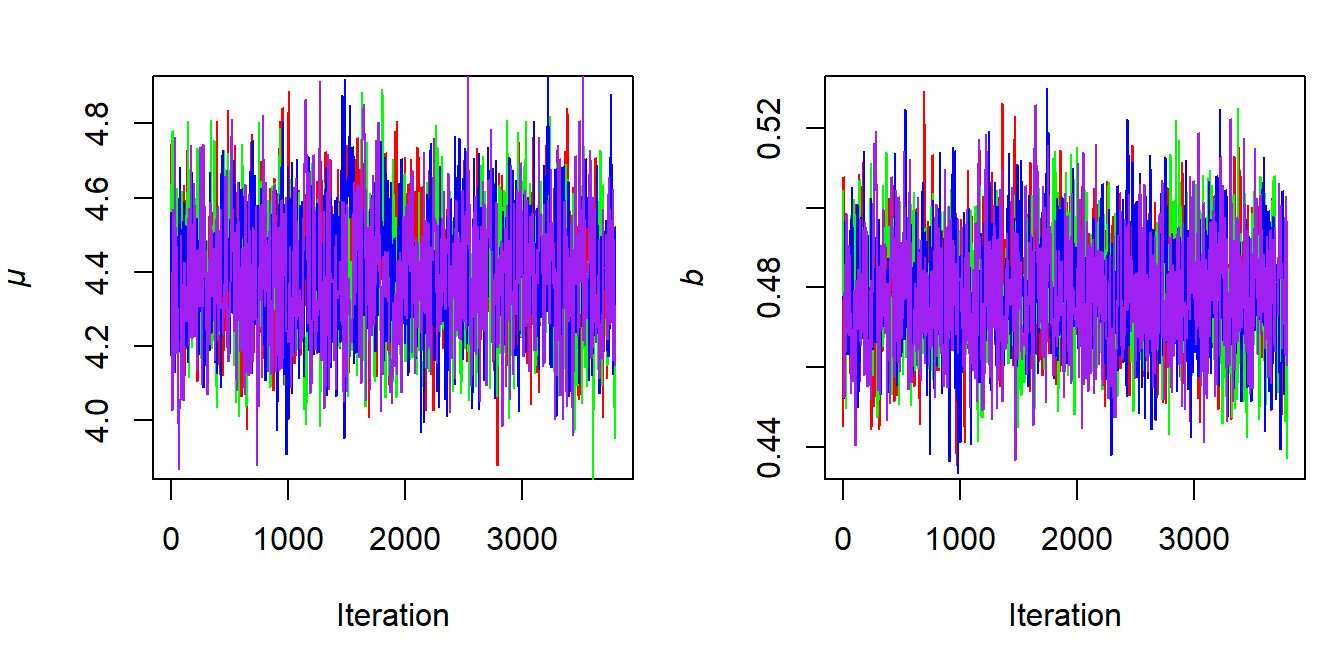
Figure 6.10: Trace plots for the multiple MCMC chains shown in Figure 6.9 after discarding the first 200 iterations as burn-in.

Well-converged chains should show no obvious trends or drifts and should resemble a “fuzzy caterpillar,” fluctuating around a stable mean. Specifically, from Figure 6.10, we can observe two properties that valid and converged MCMC runs should exhibit: mixing and stationarity.

Mixing means that the chains are sampling from the same target distribution and therefore appear well-mixed. That is, all chains are in the exact same area of high posterior probability and we cannot keep them apart unless we plot each chain in a separate color or line type. Stationarity means that the chains fluctuate around a stable mean, without exhibiting clear upward or downward trends. Lack of stationarity may indicate an ill-defined posterior distribution or an ongoing burn-in phase.

Often, visual inspection is complemented by calculating the Gelman–Rubin statistic, denoted as \(\hat{R}\). This statistic assesses convergence by comparing the variance between chains to the variance within each chain. When all chains have mixed well, \(\hat{R}\) values should be close to 1, ideally below 1.1. A common refinement is to calculate \(\hat{R}\) after splitting each chain into two halves. This allows the statistic to detect drifts: if the two halves differ substantially, the between-chain variance will increase, leading to a larger \(\hat{R}\).

6.2.4.2 Autocorrelation

In MCMC sampling, autocorrelation refers to the dependency between successive samples in a Markov chain. Although each step only depends directly on the previous one, the chain moves gradually across the parameter space. As a result, samples that are close together in time tend to be more similar than samples that result from more distal time points. This leads to correlated samples, with the correlation decaying as the temporal lag increases. Autocorrelation is a technical challenge, because it contrasts with the ideal of having independent samples from the posterior. When autocorrelation is high, the chain traverses the parameter space slowly, which can reduce the efficiency of the sampling process.

In practical terms, high autocorrelation reduces the effective sample size of the chain, meaning that we have fewer independent pieces of information for estimating posterior quantities. This may result in less precise estimates and wider credibility intervals. Fortunately, autocorrelation does not invalidate parameter estimation; it simply implies that longer-running chains are needed to gather a sufficient number of effective (i.e., quasi-independent) samples. To evaluate autocorrelation, we can inspect autocorrelation plots, which show how correlation drops off as a function of lag. In addition, we can compute the effective sample size (ESS), which corrects the total number of samples based on the estimated autocorrelation across iterations.

6.2.5 DE-MCMC

With our basic understanding of MCMC algorithms, we can now introduce a specific variant that has proven especially useful for estimating complex cognitive models like the DDM (e.g., Evans and Servant 2022). This algorithm is called Differential Evolution MCMC (DE-MCMC) (Braak 2006). It combines the Metropolis MCMC algorithm with the logic of Differential Evolution (DE).

Specifically, DE-MCMC maintains a population of chains, each representing a different point in the parameter space. Proposals for each chain are generated using differences between other population members, as in DE. However, unlike classical DE, proposals are not automatically accepted; instead, they are subject to the Metropolis acceptance criterion.

6.2.5.1 Basic steps of DE-MCMC

1. Initialize a population of \(N\) chains: Generate \(N\) parameter combinations scattered across the parameter space. These serve as the starting points of \(N\) MCMC chains. Typically, \(N\) is at least \(2d\), where \(d\) is the number of parameters.

2. Iterate through each chain and propose updates:

   2.1 For each chain \(k \in \{1, \dots, N\}\) at generation/iteration \(g\), randomly select two other chains \(r1\) and \(r2\) (\(k \neq r1\), \(k \neq r2\), \(r1 \neq r2\)). Then generate a proposal for chain \(k\) as \[\theta_k^* = \theta_{k,g} + \gamma \cdot (\theta_{r1,g} - \theta_{r2,g}) + \epsilon\,.\] Here…

   • \(\gamma\) is a scaling factor (analogous to \(F\) in DE), typically set to \(\gamma = \frac{2.38}{\sqrt{2d}}\), and
   • \(\epsilon\) is a small random noise vector (e.g., drawn from a uniform distribution) added to ensure that chains do not collapse to identical values.

   2.2 Evaluate the Metropolis acceptance ratio \[r = \frac{p(\theta_k^* | y)}{p(\theta_{k,g} | y)}\,.\] If the proposal is accepted, set \(\theta_{k,g+1} = \theta_k^*\); otherwise, keep \(\theta_{k, g+1} = \theta_{k,g}\).

   2.3 Repeat steps 2.1–2.2 for all chains.

3. Repeat step 2 for the desired number of generations, discarding an initial burn-in phase if needed.

Although DE-MCMC borrows the idea of generating proposals from the DE algorithm, there is a key difference: in the typical DE strategy, proposals for a member \(k\) are generated entirely from other members, meaning the current state of \(k\) is not involved in forming its own proposal. In contrast, DE-MCMC generates the proposal from the current state of chain \(k\) to ensure that the process satisfies the Markov property (i.e., the next state depends only on the current state). Without this, the algorithm would not define a valid Markov chain.

A key strength of DE-MCMC is that it requires only a single tuning parameter, \(\gamma\), which is typically set to \(\frac{2.38}{\sqrt{2d}}\). This makes the algorithm relatively easy to configure. In contrast to the standard Metropolis algorithm, DE-MCMC does not require manually specifying the scale of the jump distribution for proposal generation.

Additionally, because the DE update mechanism allows the population to adapt dynamically to the shape of the posterior distribution, DE-MCMC can outperform the Metropolis algorithm, especially in cases where parameters are correlated (Turner et al. 2013).

6.2.5.2 Demonstration

The following function provides a simple implementation of the DE-MCMC algorithm, tailored to our working example of estimating the drift rate \(\mu\) and boundary separation \(b\) in the classical Ratcliff DDM.

# init_lower, init_upper => space for drawing the initial population (for mu and b)
# gamma => scales the difference for generating the proposal
# epsilon => controls the size of the small noise added to the proposal
# samples => how many samples (after burn_in) shall be obtained?
# burn_in => how long should the burn-in period be?
my_de_mcmc <- function(init_lower = c(0, 0.2), init_upper = c(8, 0.9),
                       gamma = 2.38 / sqrt(4), epsilon = 0.01, samples = 500,
                       burn_in = 100) {
  d <- length(init_lower)
  pop_size <- 5 * d
  idxs <- seq_len(pop_size)
  max_iter <- samples + burn_in

  # Initialize the population
  pop <- replicate(pop_size, runif(d, init_lower, init_upper))
  posterior_vals <- apply(pop, 2, calc_posterior)

  # Store the full MCMC history for each chain
  all_samples <- array(NA, dim = c(max_iter, d, pop_size))

  for (i in 2:max_iter) {
    for (k in idxs) {
      # Select 2 other chains distinct from k
      idxs_i <- idxs[-k]
      r12 <- sample(idxs_i, 2)
      x1 <- pop[, r12[1]]
      x2 <- pop[, r12[2]]

      # Differential evolution proposal with added noise
      theta_prev <- pop[, k]
      theta_star <- theta_prev + gamma * (x1 - x2) +
        runif(d, min = -epsilon, max = epsilon)

      # calculate the posterior (cac_posterior might crash for unreasonable values,
      # so put it into a tryCatch statement)
      posterior_star <- tryCatch(
        calc_posterior(theta_star),
        error = function(err) -Inf
      )

      # Compute acceptance probability
      posterior_prev <- posterior_vals[k]
      accept_ratio <- posterior_star / posterior_prev
      r <- min(1, accept_ratio)

      # Accept or leave as is
      if (runif(1) < r) {
        pop[, k] <- theta_star
        posterior_vals[k] <- posterior_star
      }
    }
    # store the state of the population
    all_samples[i, , ] <- pop
  }

  # Discard burn-in and return all the samples
  all_samples <- all_samples[(burn_in + 1):max_iter, , ]
  return(all_samples)
}

Let us run it and plot the traces of the chains. From Figure 6.11, we can now see that the chains successfully converge to the same region of high posterior density as in the previous Metropolis algorithm.

all_samples <- my_de_mcmc() # returns array of dim samples x parameters x chains

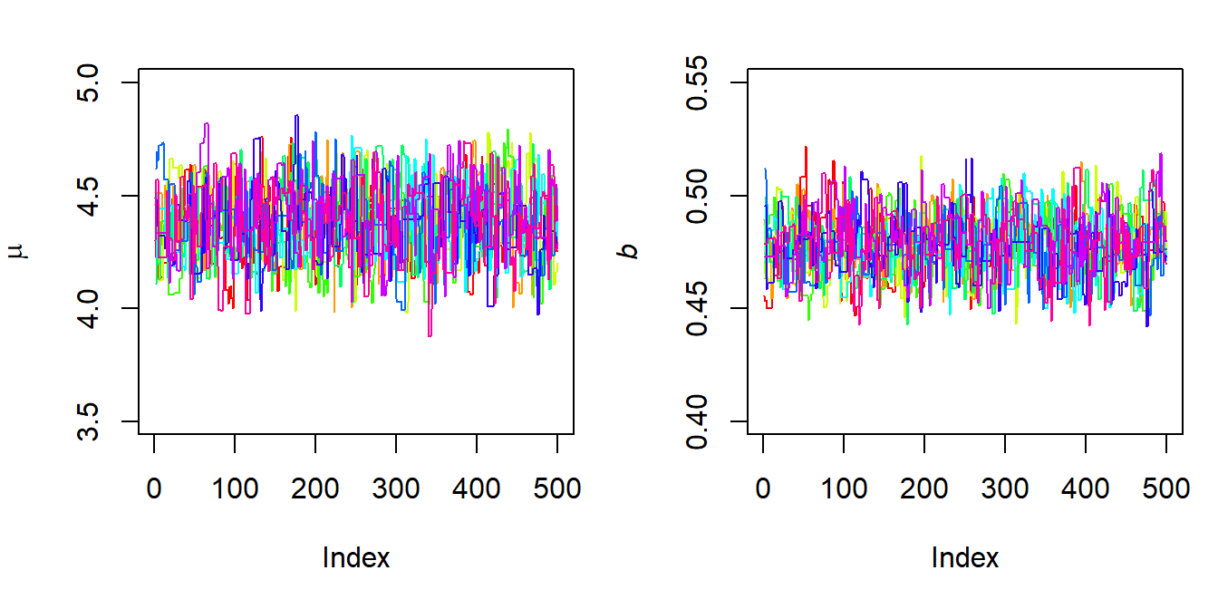
Figure 6.11: Chains of the DE-MCMC implementation.

6.2.6 Hierarchical Estimation of DDMs with DE-MCMC

One of the great strengths of the Bayesian framework is its natural ability to handle hierarchical data structures. While hierarchical parameter estimation is also possible in frequentist frameworks (see the lme4 package for regression models, Bates et al. 2015), it is often more cumbersome there, particularly because it requires to construct and optimize complex log-likelihood functions.

6.2.6.1 Building a Hierarchical Structure

But what does hierarchical actually mean in the context of DDMs? A hierarchical (or multilevel) data structure refers to data that are organized at more than one level, with lower-level units nested within higher-level groups. This structure arises naturally when observations are grouped meaningfully; most commonly, when we collect RT data from multiple participants.

In this setting, we do not estimate parameters for each individual independently. Instead, we estimate them relative to a group, which allows us to…

• simultaneously estimate model parameters at both the individual level (e.g., each participant’s drift rate) and the group level (e.g., the population-average drift rate), and to

• constrain individual parameter estimates relative to the group-level distribution. When individual data are sparse or noisy, estimates at the individual level tend to exhibit excessively high variance. By estimating each individual relative to the group, we effectively shrink extreme values toward the group mean, which improves parameter precision.

Let us consider how this structure is formalized in the context of DDMs. For simplicity of notation, let \(\theta_i^{(j)}\) denote the \(j\)-th parameter (e.g., drift rate, boundary, etc.) for participant \(i\). At the group level, we assume that each individual’s parameter is drawn from a distribution defined by group-level parameters. A common choice is the truncated normal distribution:

\[\begin{equation} \theta_i^{(j)} \sim NT(\eta^{(j)}, \sigma^{(j)}, L^{(j)}, U^{(j)})\,. \tag{6.2} \end{equation}\]

This is a reasonable assumption, as DDM parameters often follow an approximately normal distribution across participants. Additionally, the truncated normal provides a convenient way to specify

• a group-level mean \(\eta^{(j)}\) and standard deviation \(\sigma^{(j)}\), and
• lower and upper bounds \(L^{(j)}\) and \(U^{(j)}\) to constrain parameters to plausible ranges.⁴⁴

For example, if \(\theta^{(j)}\) represents the drift rate \(\mu\), the group-level distribution gives us a way to estimate both the average drift rate across participants and the variability in drift rates between individuals.

Figure 6.12 illustrates this logic. It shows a fictitious set of 10 individuals, each with their own parameter value \(\theta_i^{(j)}\). These values are assumed to have been drawn from a normal distribution with group-level parameters \(\eta^{(j)}\) and \(\sigma^{(j)}\). Additionally, for each individual, we observe a set of choice-RT data \(y_i\), which are generated based on the individual-specific parameter \(\theta_i^{(j)}\).

Figure 6.12: Illustration of group-level and individual-level parameters.

Note that the group-level parameters that govern the distribution of individual-level parameters are often referred to as hyperparameters in the Bayesian context. We denote them as \(\phi^{(j)}\), representing a tuple containing the mean and standard deviation of parameter \(j\), that is, \(\phi^{(j)} = (\eta^{(j)}, \sigma^{(j)})\).

As in any Bayesian analysis, our goal is to estimate the posterior distribution of the parameters given the data. In Section 6.2, we introduced the unnormalized posterior for a single parameter vector \(\theta\) from one participant,

\[p(\theta | y) \propto p(y | \theta) p(\theta)\,.\] In the hierarchical case, we must account for…

• all individuals, each with their own parameter set \(\theta_i\), and
  
• the group-level hyperparameters \(\phi^{(j)}\) for each model parameter.

Let \(\Theta\) be the set of all individual-level parameters and \(\Phi\) the set of all group-level hyperparameters. The (unnormalized) joint posterior for the hierarchical case then becomes \[\begin{align*} p(\Theta, \Phi|Y) &\propto p(Y|\Theta,\Phi) \cdot p(\Theta,\Phi) \\ &\propto p(Y|\Theta,\Phi) \cdot p(\Theta|\Phi) \cdot p(\Phi)\,. \end{align*}\]

Here, \(Y\) denotes all observed data across individuals. Assuming that \(\Phi\) influences the data \(Y\) only through the individual parameters \(\Theta\), we can simplify the likelihood term to depend solely on \(\Theta\), that is,

\[\begin{align*} p(\Theta, \Phi|Y) \propto p(Y|\Theta) \cdot p(\Theta|\Phi) \cdot p(\Phi)\,. \end{align*}\]

This is a typical way to express the joint posterior of a hierarchical model. However, a challenge with this general formulation, especially for complex models like the DDM, is that it involves many parameters and multiple joint distributions. For instance, the term \(p(\Theta | \Phi)\) represents the joint prior distribution over all individual-level parameters, conditional on all the group-level parameters. To manage this complexity, we often introduce simplifying assumptions, particularly assumptions of independence.

In fact, we have already implicitly introduced one such simplification when outlining the basic idea of a hierarchical model: we assumed that each individual parameter \(\theta_i^{(j)}\) has its own separate prior distribution, which effectively treats these parameters as conditionally independent given the group-level parameters. Additionally, in most experimental contexts, it is reasonable to assume that the data of different individuals are independent.

Under these assumptions, we can factorize the joint distributions into a series of products that run over each participant \(i \in \{1, \dots, N\}\) and each model parameter \(j \in \{1, \dots, P\}\)

\[\begin{align} p(\Theta, \Phi|Y) \propto \Pi_{i=1}^N p(y_i|\theta_i) \cdot \Pi_{i=1}^N \Pi_{j=1}^P p(\theta_i^{(j)}|\phi^{(j)}) \cdot \Pi_{j=1}^P p(\phi^{(j)})\,. \end{align}\]

In this equation

• \(p(y_i | \theta_i)\) is the likelihood for individual \(i\) given their parameter combination \(\theta_i = (\theta_i^{(1)}, ..., \theta_i^{(P)})\).⁴⁵
• \(p(\theta_i^{(j)} | \phi^{(j)})\) is the prior for an individual parameter \(j\) based on the group-level hyperparameters for this parameter (see also Equation (6.2)).
• \(p(\phi^{(j)})\) is the prior for the group-level mean and standard deviation of parameter \(j\).

The first and second part can be computed using the first-passage time of a DDM and the prior distributions at the individual-level. The only missing aspect is the right-most part of the (joint) prior distribution, \(p(\phi^{j})\), for a set of group-level parameters \(\phi^{j}\).

In the context of evidence accumulation models, it is common to assume that the joint prior \(p(\phi^{j})\) results from a set of independent prior distributions for each parameter in \(\phi^{j}\). That is, in our case, we specify \(p(\phi^{j}) = p(\eta^{(j)}) \cdot p(\sigma^{(j)})\). Specifically, For the group-level means \(\eta^{(j)}\), truncated normal distributions are often used (Evans and Servant 2020; Turner et al. 2013; Heathcote et al. 2019):

\[\begin{align} \eta^{(j)} \sim NT(M^{(j)}, S^{(j)}, L^{(j)}, U^{(j)}) \,. \end{align}\]

Here, \(M^{(j)}\) and \(S^{(j)}\) define the prior mean and variance, while \(L^{(j)}\) and \(U^{(j)}\) are truncation bounds, typically the same bounds used for the corresponding individual-level parameters.

For the group-level standard deviations \(\sigma^{(j)}\), gamma distributions or exponential distributions are commonly used. If we use a gamma prior, then we can write

\[\begin{align} \sigma^{(j)} \sim \Gamma(Sh^{(j)}, Ra^{(j)})\,, \end{align}\]

were \(Sh^{(j)}\) and \(Ra^{(j)}\) are shape and rate parameters chosen by the researcher. For example, Evans and Servant (2020) and Turner et al. (2013) used a shape and rate parameter of 1.

Combining all these components, the posterior for all of our individual- and group-level parameters finally becomes:

\[\begin{align} p(\Theta, \Phi|Y) \propto \Pi_{i=1}^N p(y_i|\theta_i) \cdot \Pi_{i=1}^N \Pi_{j=1}^P p(\theta_i^{(j)}|\eta^{(j)}, \sigma^{(j)}) \cdot \Pi_{j=1}^P p(\eta^{j}) \cdot \Pi_{j=1}^P p(\sigma^{j}) \,. \end{align}\]

While this decomposition breaks the complex joint posterior into manageable parts, sampling from it via MCMC still remains challenging due to its high dimensionality.

6.2.6.2 Blocked Sampling for Hierarchical Models

To manage complexity, block updating is commonly used. Rather than updating all parameters simultaneously, subsets (blocks) of parameters are updated sequentially. Geometrically, this can be thought of as slicing through the joint posterior and sampling within each slice.

A first separation is made between the individual-level and the group-level parameters. That is, we first update the group-level parameters while holding the individual-level parameters fixed. Then, we update the individual-level parameters while keeping the group-level parameters fixed.

Additional blocks are also typically formed within each level:

• At the group-level, each \(\phi^{(j)}\) is usually updated in turn. In the context of DDMs, this means that the mean and standard deviation components of \(\phi^{(j)} = (\eta^{(j)}, \sigma^{(j)})\) are updated jointly, but one parameter \(j\) at a time.

• At the individual level, the parameter combination \(\theta_i\) for each individual is typically updated sequentially, one participant at a time. This is feasible because, under the assumption of independence, the individual parameters do not influence each other directly.

Thus, in each MCMC iteration, we alternate between sampling from:

• The posterior of the group-level parameters (given the current individual-level values), that is,

\[p(\phi^{(j)}|\theta^{(j)}) \propto \Pi_{i=1}^N p(\theta_i^{(j)}|\eta^{(j)}, \sigma^{(j)}) \cdot p(\eta^{(j)}) \cdot p(\sigma^{(j)}) \,,\]

• and the posterior of the individual-level parameters (given the group-level values), that is,

\[\begin{align*} p(\theta_i | y_i, \Phi) \propto p(y_i|\theta_i) \cdot \Pi_{j=1}^P p(\theta_i^{(j)}|\eta^{(j)}, \sigma^{(j)}) \,. \end{align*}\]

6.2.6.3 Pseudo-Code for Hierarchical DE-MCMC

Extending the Bayesian framework to hierarchical data is conceptually straightforward, but as the previous section showed, it introduces several new challenges. Specifically, we must now manage multiple levels of parameters and work with different conditional posterior distributions.

We will not provide full R code here, as a complete manual implementation would become quite verbose and offers little conceptual gain. Instead, we present pseudo-code: a simplified, informal way of describing an algorithm that focuses on logic rather than strict programming syntax. This allows us to emphasize the structure of hierarchical DE-MCMC without being distracted by implementation details.

INPUT:
  - Number of chains \(K\), iterations \(G\)
  - individual data sets \(y_i = (y_1, \dots, y_N)\)

OUTPUT:
  - Posterior samples for group-level parameters \(\Phi\) and individual-level parameters \(\Theta\)

INITIALIZE:
FOR EACH chain \(k\) in \((1, \dots,K)\)
  Sample initial group-level parameters \(\phi_{k,1}^{(j)}\) for all \(j\) to build \(\Phi_{k,1}\)
FOR EACH individual \(i\) in \((1, \dots, N)\)
  Sample initial parameters \(\theta_{i,k,1}^{(j)}\) for all \(j\) to build \(\theta_{i,k,1}\)


SAMPLING:
FOR EACH iteration \(g\) in \((2, \dots, G)\)
  FOR EACH chain \(k\) in \((1, \dots, K)\)
    FOR EACH parameter \(j\) in \((1, \dots, P)\)
      Select two other chains \(r1 \neq r2 \neq k\)
      Propose:
     \(\phi_*^{(j)} = \phi_{k,g-1}^{(j)} + \gamma \cdot (\phi_{r1,g-1}^{(j)} - \phi_{r2,g-1}^{(j)}) + \epsilon\)
      Compute acceptance ratio:
     \(r = \min\left(1, \frac{p(\phi_*^{(j)} | \theta_{k,g-1}^{(j)})}{p(\phi_{k,g-1}^{(j)} | \theta_{k,g-1}^{(j)})} \right)\)
      IF \(r > \text{Uniform}(0,1)\):
       \(\phi_{k,g}^{(j)} \leftarrow \phi_*^{(j)}\)
      ELSE
       \(\phi_{k,g}^{(j)} \leftarrow \phi_{k,g-1}^{(j)}\)

  FOR EACH individual \(i\) in \((1, \dots, N)\)
    FOR EACH chain \(k\) in \((1, \dots,K)\)
      Select two other chains \(r1 \ne r2 \ne k\)
      Propose:
     \(\theta_{i,*} = \theta_{i,k,g-1} + \gamma \cdot (\theta_{i,r1,g-1} - \theta_{i,r2,g-1}) + \epsilon\)
      Compute acceptance ratio:
     \(r = \min\left(1, \frac{p(\theta_{i,*} | y_i, \Phi_{k,g-1})}{p(\theta_{i,k,g-1} | y_i, \Phi_{k,g-1})} \right)\)
      IF \(r > \text{Uniform}(0,1)\):
       \(\theta_{i,k,g} \leftarrow \theta_{i,*}\)
      ELSE
       \(\theta_{i,k,g} \leftarrow \theta_{i,k,g-1}\)

6.2.7 Exercise: Bayesian Estimation of DMC

1.) Load the flanker data set of Ulrich et al. (2015) and fit DMC to individual 9 using differential evolution and dRiftDM (call ?estimate_model for aid). Have a look at the parameter estimate of the peak latency \(\tau\). How do you judge this estimate against the background of typical \(\tau\) values in a flanker task? Visualize the fitted delta function.

2.) Now fit the same data set of individual 9 once more but with the function estimate_model_bayesian() of dRiftDM. Use 300 iterations as burn-in, 300 samples, and 40 chains. Define your own set of priors for each model parameter. How to do this can be obtained from the documentation and the respective examples. The function returns the posterior samples and you can get a summary of the posterior samples like this:

samples <- estimate_model_bayesian(...)
coef(samples)

How did the Bayesian approach to parameter estimation change the parameter estimates? Addition: Use the generic summary() and plot() methods to explore the posterior samples.

3.) Estimate the entire data set using a hierarchical Bayesian approach to parameter estimation and a more classical approach of fitting each individual independently. Compare the parameter estimates. What effect can you observe?

6.2.8 Final Comments on Model Checking

In the previous sections, we have focused on the technical aspects of estimating the parameters of a model within the Bayesian framework focusing on MCMC algorithms and how they work. Of course, this is only a first glimpse on the Bayesian inference machine. Thus, before closing the section, we want to highlight additional steps that should be performed for a fully Bayesian approach to modeling, to ensure the integrity of any conclusions. Three particularly useful techniques are prior predictive checks, posterior predictive checks, and sensitivity analyses.

1. A prior predictive check answers the question: “What kind of data would my model produce before seeing any actual data?” To this end, we…

   • sample parameter values only from the prior distributions,
   • generate simulated data using those sampled parameters and the model’s predicted PDF, and
   • compare the simulated data to what we would expect from real experiments (e.g., plausible RT ranges, error rates, delta function shapes).

   This helps us evaluate whether our priors are reasonable or too restrictive/unrealistic. For example, if the prior predictive distribution leads to implausibly short or long RTs, we might reconsider the ranges or shape of our prior distributions.

2. A posterior predictive check asks: “Given what I have learned from the data, can my model reproduce the observed patterns?” To this end, we

   • use samples from the posterior distribution (i.e., parameters that fit the data well),
   • simulate new data based on these parameters, and
   • compare the simulated data to the actual observed data (e.g., using histograms of RT distributions, quantiles or delta functions).

   This help us evaluate how well the model captures key features of the empirical data. If the posterior predictive simulations deviate systematically from the observed data (e.g., the model underpredicts or overpredicts the observed delta function), this suggests the model may be misspecified or missing a key component. Of course, this kind of model checking is a fundamental part of any cognitive modeling exercise, and not limited to the Bayesian framework. We have already emphasized in previous exercises, and, especially when introducing conflict diffusion models: A good model should not only match the data well, but also reproduce critical qualitative patterns in the data.

3. In Bayesian inference, results are influenced not only by the observed data, but also by the prior distributions. While this is one of the strengths of the Bayesian approach (as it allows incorporating prior knowledge), it also means that the conclusions may depend on the specific priors chosen. Sensitivity analysis helps to assess the robustness of the results to these choices. To this end, we…

   • re-fit our model under different plausible priors, which differ in their location, scale, or shape, and
   • check how much the posterior inferences change.

   If our conclusions remain stable across a reasonable range of prior settings, our inferences are said to be robust. If they vary substantially, they are sensitive to the priors, and should be interpreted accordingly.

6.3 Solutions for the Exercises

6.3.1 Exercise: Simplex vs. Differential Evolution

rm(list = ls())

# create the model and set a seed
ssp <- ssp_dm(dx = 0.002, dt = 0.002, t_max = 3.0, var_non_dec = FALSE)
set.seed(1)

# simulate the data
synth_data_prms <- simulate_data(
  object = ssp, n = 100, k = 50,
  lower = c(b = 0.35, non_dec = 0.20, p = 2.0, sd_0 = 1.0),
  upper = c(b = 0.95, non_dec = 0.45, p = 5.5, sd_0 = 2.6)
)

# increase discretization
prms_solve(ssp)["dx"] <- 0.01
prms_solve(ssp)["dt"] <- 0.01


# now try to recover the parameters using Nelder-Mead
estimate_model_ids(
  drift_dm_obj = ssp, obs_data_ids = synth_data_prms$synth_data,
  lower = c(b = 0.35, non_dec = 0.20, p = 2.0, sd_0 = 1.0),
  upper = c(b = 0.95, non_dec = 0.45, p = 5.5, sd_0 = 2.6),
  fit_procedure_name = "recov_ssp_nm",
  fit_path = getwd(),
  use_de_optim = FALSE, 
  use_nmkb = TRUE
)

# now try to recover the parameters using Differential Evolution (default)
estimate_model_ids(
  drift_dm_obj = ssp, obs_data_ids = synth_data_prms$synth_data,
  lower = c(b = 0.35, non_dec = 0.20, p = 2.0, sd_0 = 1.0),
  upper = c(b = 0.95, non_dec = 0.45, p = 5.5, sd_0 = 2.6),
  fit_procedure_name = "recov_ssp_de",
  fit_path = getwd(),
  de_n_cores = 4 # use 4 cores/threads for parallelization
)

# load the fits and store get the parameter estimates
prms_nm <- coef(load_fits_ids(fit_procedure_name = "recov_ssp_nm"))
prms_de <- coef(load_fits_ids(fit_procedure_name = "recov_ssp_de"))
prms_orig <- synth_data_prms$prms

# finally, plot the parameters
par(mfrow = c(2, 2))
for (i in names(coef(ssp))) {
  plot(prms_orig[[i]] ~ prms_nm[[i]],
    ylab = "Original", xlab = "recovered",
    main = i
  )
  points(prms_orig[[i]] ~ prms_de[[i]], col = "red")
}
legend("bottomright", legend = c("Nelder-Mead", "DE"), col = c("black", "red"), 
       pch = 21)

Both approaches yield very similar estimates! This suggests that Nelder–Mead works quite well for fitting the SSP model, at least with the current starting values, parameter ranges, and trial numbers.⁴⁶

6.3.2 Exercise: Bayesian Estimation of DMC

1.)

rm(list = ls())

# get the data and the model
data <- dRiftDM::ulrich_flanker_data
one_subj <- data[data$ID == 9, ]
dmc_model <- dmc_dm(t_max = 1.5, dt = .01, dx = .01, obs_data = one_subj)

# estimate the model
dmc_est_clas <- estimate_model(
  dmc_model,
  lower = c(1, 0.2, 0.1, 0.01, 0.01, 0, 2),
  upper = c(8, 1.0, 0.5, 0.10, 0.25, 0.3, 8),
  de_n_cores = 3
)

# what is the estimate for tau?
round(coef(dmc_est_clas), 3)

##        muc          b    non_dec sd_non_dec        tau          A      alpha 
##      4.060      0.532      0.301      0.025      0.250      0.127      8.000

# the delta function
plot(
  calc_stats(
    dmc_est_clas,
    type = "delta_funs",
    minuends = "incomp", subtrahends = "comp"
  )
)

When estimating individual 9 in isolation, we obtain a very high \(\tau\) value, which lies at the upper end of the specified parameter space. Given the shape of the observed delta function, this makes sense. However, it is important to note that \(\tau\) is known to be difficult to estimate when the delta function is steep, and it is not uncommon for \(\tau\) to “drift” toward higher values.

2.)

set.seed(1)
samples <- estimate_model_bayesian(
  drift_dm_obj = dmc_model,
  burn_in = 300, 
  samples = 300,
  mean = c(tau = 0.12),
  sd = c(tau = 0.06),
  lower = c(tau = 0.01)
)

##        muc          b    non_dec sd_non_dec        tau          A      alpha 
##      4.060      0.532      0.301      0.025      0.250      0.127      8.000

##        muc          b    non_dec sd_non_dec        tau          A      alpha 
##      4.055      0.538      0.300      0.026      0.168      0.103      9.005

When using a Bayesian approach, we can define a prior over \(\tau\), for example, specifying that we expect \(\tau\) values to be around 0.12 seconds in a typical flanker task. This prior belief acts as a constraint during estimation and helps to stabilize the resulting parameter estimates. In the case of participant 9, the posterior mean of \(\tau\) ends up way closer to the prior’s mean, effectively pulling the estimate toward a more plausible range and reducing the risk of overestimation.

We can get trace plots by supplying samples to the generic plot() method:

par(mfrow = c(3,3))
plot(samples)

A summary on the chains can be obtained via summary():

summary(samples)

## Sampler: de_mcmc 
## Hierarchical: FALSE 
## No. Parameters: 7 
## No. Chains: 40 
## Iterations Per Chain: 300 
## 
## -------
## Parameter Summary: Basic Statistics
##             Mean    SD Naive SE Time-series SE
## muc        4.055 0.242    0.002          0.011
## b          0.538 0.036    0.000          0.002
## non_dec    0.300 0.007    0.000          0.000
## sd_non_dec 0.026 0.003    0.000          0.000
## tau        0.168 0.047    0.000          0.002
## A          0.103 0.027    0.000          0.001
## alpha      9.005 2.532    0.023          0.109
## 
## Gelman-Rubin Statistics
##        muc          b    non_dec sd_non_dec        tau          A      alpha 
##      1.028      1.044      1.049      1.042      1.044      1.061      1.052 
## 
## Effective Sample Size
##        muc          b    non_dec sd_non_dec        tau          A      alpha 
##    568.678    586.177    595.683    615.946    596.060    644.949    657.957

3.)

# get the data and a fresh model object
data <- dRiftDM::ulrich_flanker_data
dmc_model <- dmc_dm(t_max = 1.5, dt = .01, dx = .01)

# estimate DMC in the classical way
estimate_model_ids(
  drift_dm_obj = dmc_model,
  obs_data_ids = data,
  lower = c(1, 0.2, 0.1, 0.01, 0.01, 0, 2),
  upper = c(8, 1.0, 0.5, 0.10, 0.25, 0.3, 8),
  fit_procedure_name = "flanker_dmc",
  fit_path = getwd(),
  de_n_cores = 4, 
  seed = 1
)


# estimate DMC using a hierarchical Bayesian approach
samples_h <- estimate_model_bayesian(
  drift_dm_obj = dmc_model,
  obs_data_ids = data,
  burn_in = 500,
  samples = 500,
  mean = c(tau = 0.12),
  lower = c(tau = 0.01), 
  seed = 1
)

# get the parameter estimates of the classical approach
all_fits <- load_fits_ids(fit_procedure_name = "flanker_dmc")
prms_class <- coef(all_fits)

# get average parameter estimates for the hierarchical approach
prms_bayes = coef(samples_h, id = NA)

# now compare
par(mfrow = c(3, 3))
for (i in names(coef(dmc_model))) {
  bayes <- prms_bayes[[i]]
  class <- prms_class[[i]]
  ax_min <- min(c(bayes, class))
  ax_max <- max(c(bayes, class))

  plot(bayes ~ class,
    main = i, ylim = c(ax_min, ax_max),
    xlim = c(ax_min, ax_max),
    ylab = "Bayesian estimates", xlab = "Classical estimates"
  )
  abline(coef = c(0, 1))
}

When comparing the parameter estimates, we generally observe strong agreement between the classical and hierarchical approaches. However, under the hierarchical approach, the estimates exhibit reduced variance. Specifically, estimates that tend to be small in the classical (individual) approach are often slightly larger under the hierarchical model. Conversely, estimates that tend to be large are often slightly smaller. This phenomenon is known as shrinkage: individual estimates are “pulled” toward the group-level mean. Shrinkage is a natural consequence of hierarchical modeling and helps stabilize parameter estimates, especially when individual data are noisy or sparse.

---

37. Bayesian inference is not the only approach to quantify uncertainty. For example, likelihood theory uses the Fisher information to derive confidence intervals, and bootstrapping can also be used to estimate variability. However, such methods are rarely applied in the context of diffusion modeling, likely due to numerical challenges and computational demands.↩︎

38. This is why we write \(NP\) to capture the \(N\)umber of \(P\)opulation members in accordance with the original notation of Storn and Price (1997)↩︎

39. Here, \(F = 0.8\) was used.↩︎

40. When optimization fails, it is more often due to issues with the model itself or poorly chosen search spaces, not the settings of DE.↩︎

41. Just like drawing many samples from a known distribution (e.g., rnorm(100000)) produces a histogram that approximates its density.↩︎

42. We use the symbol \(\eta\) for the expected value of this multivariate distribution to reserve \(\mu\) for the drift rate.↩︎

43. While it is possible to model a prior covariance structure among parameters in the Bayesian framework, a common approach in the context of DDMs is to assume that each parameter is independent of the others.↩︎

44. If we set the lower and upper bounds to minus infinity and infinity, respectively, we obtain the classical normal distribution.↩︎

45. This is the likelihood we have maximized so far! (or minimized, depending on how you frame the optimization problem)↩︎

46. To be honest, this was not the originally expected result when designing the exercise. We intended to demonstrate that DE is more robust than Nelder–Mead. However, it appears that the cost function for SSP is relatively smooth and does not contain many problematic local minima.↩︎