3 Getting Started: Diffusion Models Hands-On

In Chapter 1 of this book, we discussed what cognitive models are at a conceptual level and why they are useful for describing decision-making processes. We also introduced conflict tasks as typical experimental tasks in cognitive psychology, and emphasized that a cognitive model has to accurately describe the distribution of choice-RT data.

In the subsequent Chapter 2, we then discussed how we can actually model the core aspect of a response, that is the response selection or decision process that maps an initial stimulus percept to an overt response (see also again Figure 1.3). To this end, we introduced the RW and the DDM as prominent examples of the general class of sequential sampling models.

In the present chapter, we will put our theory into practice by working hands-on with dRiftDM in Section 3.1. We will also extend our basic knowledge on DDMs to cover models that are generally known as conflict DDMs; specifically, the Diffusion Model for Conflict tasks (DMC, 3.2.1) and the Shrinking Spotlight Model (SSP, Section 3.2.2). These models were explicitly developed to account for conflict task data and are characterized by a time-dependent drift rate that varies over the course of a trial (see also Section 2.3.3).

3.1 The Ratcliff DDM: Predictions and Extensions

In Sections 2.3.3 and 2.3.5, we have already developed and programmed the simplest DDM with a drift rate $\mu$, a boundary $b$, and a non-decision time $t0$. This is the model that Ratcliff (1978) utilized in the context of memory research and we will refer to it as the Ratcliff DDM.¹⁵ Although it is the simplest DDM it is already highly useful and has been successfully applied to an impressive range of different tasks (see, e.g., Ratcliff et al. 2016).

Before we get started, let’s first clarify three things to avoid confusion:

Often, we are not particularly interested in whether the “upper” or “lower” response was chosen (e.g., a left or right response, respectively). Instead, it’s common to abstract away from stimulus/response mappings and assume that the upper boundary codes a correct response, and the lower boundary an error. Consequently, the drift rate $\mu$ is assumed to be larger than zero, because otherwise participants would select more often an incorrect than correct response. This is called an accuracy coding and it is the default coding in dRiftDM.
Additionally, we assume the boundary to be symmetric, spanning the interval $[-b, b]$, just like we did when we introduced RWs and DDMs in the last chapter. This is different to some other software solutions, like fast-dm, where the boundaries span an interval $[0, a]$. In this case $a$ is called the boundary separation or threshold separation, and the center in between the boundaries is $a/2$. Importantly, this is just a matter of notation and parameterization, and does not change the model behavior.
In the following, you might encounter parameter values that seem odd against the background of the previous Chapter 2. For example, in Section 2.3.3, the drift rate was 0.2 and the boundary somewhere between 3 or 10. This is because we scaled the time and evidence space in a way that is most intuitive for introducing RWs (e.g., $\Delta t$ was 1 ms). In dRiftDM, however, the parameters are expressed in the unit of seconds, as this is most typical for DDMs. Again, this does not change the model predictions, but it just changes the relative size of parameters. In the present book, we will not cover how to convert parameters from seconds to milliseconds and how to transform parameters when the diffusion constant $\sigma$ is changed. However, interested readers can find some information on that in our online vignette for dRiftDM as well as in Ulrich et al. (2016).

To create the classical Ratcliff DDM with default settings in dRiftDM, we can call ratcliff_dm():

simple_ddm <- ratcliff_dm()

When printing the model to the console we can access basic information about it:

print(simple_ddm)

## Class(es): ratcliff_dm, drift_dm
## 
## Current Parameter Matrix:
##      muc   b non_dec
## null   3 0.6     0.3
## 
## Unique Parameters:
##      muc b non_dec
## null   1 2       3
## 
## Deriving PDFs:
##   solver: kfe
##   values: sigma=1, t_max=3, dt=0.001, dx=0.001, nt=3000, nx=2000
## 
## Observed Data: NULL

The first line of the output indicates the type of model. The next three lines show the parameters of the model and their currently set values. For example, we have the parameter muc with a corresponding value of 3. For the Ratcliff model, muc is the constant drift rate $\mu$, b the constant boundary $b$, and non_dec the constant non-decision time $t0$.

In dRiftDM, we differentiate between the currently set values for each parameter (i.e., Current Parameter Matrix), and a specification about how each parameter relates across conditions and whether a respective parameter can be estimated. This is why there is the second part of the output Unique Parameters. This part summarizes whether each parameter is considered free or fixed, that is, if it can be estimated or not. We see that there are three unique parameters in the model that can be estimated, indicated by the numbers 1-3 for muc, b, and non_dec. The specifications listed here become more relevant as we move on to fitting a model in Chapter 4 and as we dive into the details of model customization in Chapter 5.

Note that every model in dRiftDM requires condition(s) to be specified. Since the Ratcliff DDM does not depend on multiple conditions, we labeled the one and only condition as “null” to indicate that the condition is irrelevant here. We will discuss models with multiple conditions in Sections 3.2.1 and 3.2.2.

The lower part of the output shows settings relevant to the derivation of the first-passage time. The solver attribute controls the numerical approach. Per default, the option is kfe, which refers to the method discussed in Section 2.3.6. The values below should already be familiar to you. They show the diffusion constant, sigma, the maximal time of the time space, t_max, and the discretization width of the time and state/evidence space, dt and dx. The respective number of steps are shown by nt and nx, respectively. We will leave the settings for dx, dt, and t_max at default values, because we keep our focus on basic model properties for now. However, we already want to stress that these settings have a substantial influence on the time dRiftDM takes to derive model predictions. Oftentimes, we can gain a speed-up of about 10 to 100 times by making the discretization more coarse, without sacrificing too much of precision. This will be relevant once we start fitting a model to data, because, as we have loosely covered in Section 1.5, fitting a model to data requires to derive model predictions many times for various different parameter combinations (and in this case it makes a difference if a model is estimated in 1 hour or 10 hours).

The last line shows if data are attached to the model. Currently, this is not the case, as indicated by NULL.

3.1.1 Exploring Parameter Effects on RT and Accuracy

To access and alter the parameter settings, we can use the coef() method:

coef(simple_ddm)

##     muc       b non_dec 
##     3.0     0.6     0.3

coef(simple_ddm)["muc"] <- 2.5
coef(simple_ddm)

##     muc       b non_dec 
##     2.5     0.6     0.3

To derive model predictions, we can use the calc_stats() method, which we have already used to explore observed data in the exercises in Section 1.4.3. To obtain predicted mean RTs and accuracy, we provide the argument type = "basic_stats":

calc_stats(simple_ddm, type = "basic_stats")

## Type of Statistic: basic_stats
## 
##   Source Cond Mean_corr Mean_err SD_corr SD_err P_corr
## 1   pred null     0.517    0.517   0.156  0.156  0.953
## 
## (access the data.frame's columns/rows as usual)

Just like we have observed in the exercises in Section 2.2.3.2, the mean first-passage time for correct and incorrect responses is identical! Apparently, this result also generalizes to DDMs.¹⁶ Additionally, the standard deviations are identical. In fact, the entire first-passage-times for correct and incorrect responses are identical (just scaled differently, because correct responses are more common than error responses; see also Figure 2.5).

Figure 3.1 illustrates the effects of each parameter on predicted mean correct RTs (black line) and accuracy (blue lines) by systematically varying each parameter one after the other. Specifically, the default parameter settings were:

$\mu = 3$
$b = 0.6$
$t0 = 0.300$

For the left, middle, and right panel of the figure, the following parameter ranges were used (while keeping the other two parameters constant at the default values):

Drift rate: $\mu \in \{1.5, 2.0, \ldots, 4.5, 5.0\}$
Boundary: $b \in \{0.2, 0.3, \ldots, 0.8, 0.9\}$
Non-decision time: $t0 \in \{0.1, 0.15, \ldots, 0.40, 0.45\}$

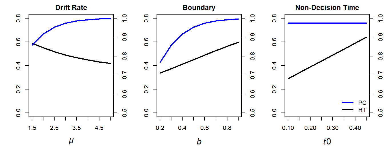
$Illustration of how $\mu$ (left panel), $b$ (middle panel), and $t0$ (right panel) change a DDM's predicted mean response times (RTs; left y-axis) and proportion correct (PC; right y-axis).$

Figure 3.1: Illustration of how $\mu$ (left panel), $b$ (middle panel), and $t0$ (right panel) change a DDM’s predicted mean response times (RTs; left y-axis) and proportion correct (PC; right y-axis).

The effects of these variations on RTs and accuracy are straightforward:

As $\mu$ increases, (1) RTs decrease and (2) accuracy increases.
As $b$ increases, (1) RTs increase and (2) accuracy increases. This reflects the well-known speed–accuracy trade-off (SAT, see Liesefeld and Janczyk 2019, 2023; Lerche and Voss 2018; Wickelgren 1977): The faster responses, the more errors are made.
As $t0$ increases, (1) RTs increase while (2) accuracy remains unchanged.

3.1.2 Extension of the Full Ratcliff Model

3.1.2.1 Additional Parameters

In the previous section, we have introduced the simplest DDM which incorporates a drift rate $\mu$, a boundary $b$, and a non-decision time $t0$. Several extensions of this model are possible.

Although we haven’t explicitly stated it, there is also the parameter $z$, which controls the starting point of the diffusion process. In the previous sections, and also in Chapter 2, we have almost always assumed that all decision processes start from the fixed value $z = 0$, which lays exactly in between the decision boundaries. However, DDMs are not limited to this assumption, and we can also assume starting value of $z \neq 0$. For example, the starting point might be closer to the upper than the lower boundary. From a psychological perspective, this shift in the starting point reflects a decision bias that is present even before the actual decision process has started.

Whether this bias is psychologically plausible depends on the context. If we model accuracy data so that the upper and lower boundaries code correct and incorrect responses, respectively, then a bias rarely makes sense. This is because participants usually can’t have a general bias for the correct or incorrect response prior to the decision process. However, it is also common to explicitly model response alternatives, so that the upper and lower boundaries directly reflect a certain response such as left or right.¹⁷ In this case, a bias for a certain response type might indeed make sense, and can be modeled using $z$. In dRiftDM, accuracy coding is the default and thus ratcliff_dm() doesn’t provide a parameter for $z$ out-of-the-box. However, it would be easy to write a custom Ratcliff DDM that does incorporate such a parameter, and we will cover model customization in Chapter 5 (see in particular Section 5.2).¹⁸

When reading about DDMs, you might have also already encountered that researchers often incorporate additional sources of variability. Specifically, three sources of additional variability are often considered, namely trial-by-trial variability

of the starting point $z$, $s_{z}$,
of the drift rate $\mu$, $s_{\mu}$, and
of the non-decision time $t0$, $s_{t0}$ (see also Section 2.3.5).

The core idea is that a participant’s cognitive architecture and motor performance is not constant, but rather varies from trial to trial. For example, participants might sometimes expect a specific stimulus and response, so that their decision is already biased toward a response in some trials (although unsystematically from trial to trial, so that the starting point is still zero on average when modeling accuracy data). Similarly, participants might be fully alert on some trials, while on others they may be daydreaming about the end of the experiment, what might end in variations of the drift rate. Thus, variability in certain parameters of a DDM is psychologically plausible.

If a DDM includes these parameters of variability, it can handle unique data patterns that the standard Ratcliff DDM cannot predict (Ratcliff and Rouder 1998). In such cases, failure to include such variability, if the data shows such patterns, can yield a mediocre fit and might even bias parameter estimates, as the model tries to fit a data pattern that it is not suited for. We will cover how each source of variability shapes the model predictions below.

To incorporate trial-by-trial variability, $z$, $\mu$, and $t0$ are not assumed to be fixed values, but rather they are conceived as random variables and their realizations for each trial are drawn from distributions. The dispersion of the respective distribution, and hence of the PDF, is described by the parameters $s_{z}$, $s_{\mu_c}$, and $s_{t0}$, respectively.¹⁹

For the starting point, the trial-by-trial variability implicates that evidence accumulation starts closer to the upper boundary on some trials and on others closer to the lower boundary. Mathematically, researchers often use a normal or uniform distribution to model the PDF of the variable starting point. In this case $s_{z}$ either captures the standard deviation or the range of the respective PDF, while $z$ describes its center (with usually $z=0$ in case of accuracy coding).

The variability in the drift rate and the non-decision time is modeled in a similar vein. Specifically, the drift rate is often assumed to follow a normal distribution with mean $\mu$ and a standard deviation $s_{\mu}$. The non-decision time is often assumed to either follow a normal distribution or uniform distribution with mean $t0$ and a standard deviation or range of $s_{t0}$, respectively.

3.1.2.2 Exploring the Effect of Variability on Model Predictions

We will now (interactively) explore how each source of variability shapes the model predictions using dRiftDM. To this end, we will plot the predicted quantiles of correct responses and the CAF of the simplest Ratcliff DDM, and compare those to an extended one, considering each source of variability one after the other.

To calculate and plot the quantiles and the CAF, we can again use a combination of calc_stats() and the generic plot() method:

# fresh simple DDM with default parameter values
simple_ddm <- ratcliff_dm() 
preds_standard <- calc_stats(simple_ddm, type = c("quantiles", "cafs"))

# plot each statistic separately to have custom axis-limits
par(mfrow = c(1, 2), cex = 1.0)

plot(preds_standard$quantiles, xlim = c(0.3, 0.7))
plot(preds_standard$cafs, ylim = c(0.5, 1))

Figure 3.2: Predicted quantiles and CAF of the simplest Ratcliff DDM.

In contrast to the output from type = "basic_stats" in Section 3.1.1, Figure 3.2 shows more information about the distribution of predicted RTs. Here, something unique is noteworthy already. For the simplest Ratcliff DDM without any additional trial-by-trial variability, predicted accuracy is always the same, irrespective of the response speed. This is clearly apparent from the CAF in the right panel of Figure 3.2. Remember that a CAF plots accuracy as function of response speed, and the exactly horizontal CAF indicates that accuracy was the same for short, intermediate, and long RTs.

Now we incorporate additional sources of variability. To this end, we make use of additional arguments of the ratcliff_dm() function. To include trial-by-trial variability of the starting point, we simply create the model by using:

var_start_ddm <- ratcliff_dm(var_start = TRUE)
coef(var_start_ddm)

##         muc           b     non_dec range_start 
##         3.0         0.6         0.3         0.5

From the parameter output it is apparent that the model now has an additional parameter range_start. This parameter corresponds to $s_{z}$ in the notation above and reflects the range of a centered uniform distribution in dRiftDM. How does this change the model predictions? To explore this, we slightly increase range_start to make its effect more prominent, and then plot the quantiles and CAF again:

coef(var_start_ddm)["range_start"] = 1
preds_var_start <- calc_stats(var_start_ddm, type = c("quantiles", "cafs"))


# plot each statistic separately to have custom axis-limits
par(mfrow = c(1, 2), cex = 1.0)

plot(preds_var_start$quantiles, xlim = c(0.3, 0.7))
plot(preds_var_start$cafs, ylim = c(0.5, 1))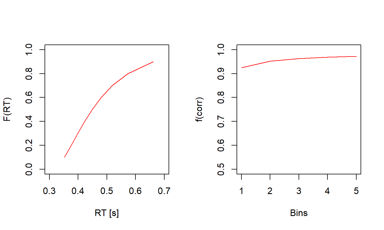

Figure 3.3: Predicted Quantiles and CAF of a Ratcliff DDM With Trial-by-Trial Variability in the Starting Point.

When comparing Figure 3.3 to Figure 3.2 it is apparent that the predicted quantiles remain almost unchanged. Yet, the CAF has clearly changed, and now reveals lower accuracy for fast responses (i.e., the CAF is slightly sloped toward the left). This indicates that those responses that are generally faster are those that are slightly more error-prone as well. Therefore, allowing the starting point to vary from trial-to-trial enables the DDM predict fast errors! Such fast errors are not uncommon for 2-AFC tasks, especially for conflict tasks. We can also see this effect in mean RTs now:

calc_stats(var_start_ddm, type = "basic_stats")

## Type of Statistic: basic_stats
## 
##   Source Cond Mean_corr Mean_err SD_corr SD_err P_corr
## 1   pred null     0.484    0.443   0.135  0.121  0.956
## 
## (access the data.frame's columns/rows as usual)

We see that the mean RT for correct responses is slightly longer than the mean RT for error responses.

Next we create a model with trial-by-trial variability of the drift rate. Again we simply use an additional argument of the ratcliff_dm() function:

var_drift_ddm <- ratcliff_dm(var_drift = TRUE)
coef(var_drift_ddm)

##     muc       b non_dec  sd_muc 
##     3.0     0.6     0.3     1.0

In this case the model now includes the parameter sd_muc, which corresponds to the standard deviation $s_{\mu}$ of a normal distribution with mean muc/$\mu$. Plotting again the quantiles and the CAF reveals its influence:

Figure 3.4: Predicted Quantiles and CAF of a Ratcliff DDM With Trial-by-Trial Variability in the Drift Rate.

From Figure 3.4 it is apparent that variability of the drift rate leads to lower accuracy for slow responses (i.e., the CAF is slightly sloped to the right). Therefore, including variability in the drift rate enables a DDM to predict slow errors! This is again also apparent in the mean RTs, where we see that mean error RTs are now slightly longer than mean correct RTs.

calc_stats(var_drift_ddm, type = "basic_stats")

## Type of Statistic: basic_stats
## 
##   Source Cond Mean_corr Mean_err SD_corr SD_err P_corr
## 1   pred null     0.495    0.556   0.152  0.207  0.952
## 
## (access the data.frame's columns/rows as usual)

In essence, we can summarize so far that variability in the starting point and drift rate lead to fast and slow error responses, respectively. These patterns are not uncommon in empirical data. The final source of variability is that of the non-decision time, which we include by creating the model as:

var_non_dec_ddm <- ratcliff_dm(var_non_dec = TRUE)
coef(var_non_dec_ddm)

##           muc             b       non_dec range_non_dec 
##          3.00          0.60          0.30          0.05

In this case the model no included the parameter range_non_dec, which corresponds to the range $s_{t0}$ of a uniform distribution with mean non_dec/$t0$. To see its impact, we again first increase the respective parameter and subsequently plot the quantiles and the CAF. From Figure 3.5 it is apparent that the variability in the non-decision time does not alter the CAF. This makes sense, because whether a response is correct or incorrect is determined during the decision component of a DDM, and not during the non-decision time. However, when comparing the distribution of quantiles in Figure 3.5 (left panel) to that in Figure 3.2 (left panel), it becomes clear that the width of RTs has increased. Thus, incorporating trial-by-trial variability in the non-decision time enables a DDM to predict a broader RT distribution.

Figure 3.5: Predicted Quantiles and CAF of a Ratcliff DDM With Trial-by-Trial Variability in the Non-Decision Time.

3.1.3 Final Remark and Summary

To summarize, the simplest Ratcliff DDM has three parameters: the drift rate $\mu$, the boundary $b$, and the non-decision time $t0$. If we include additional sources of variability of the starting point, drift rate, and non-decision time, the Ratcliff DDM may include three more parameters, in particular $s_{\mu}$, $s_z$, and $s_{t_0}$. Finally, if we also allow the (average) starting point to vary freely rather than fixing it midway between the boundaries at $z = 0$, the Ratcliff DDM includes a total of seven parameters: $\mu$, $b$, $t0$, $z$, $s_{\mu}$, $s_z$, and $s_{t_0}$ . This model is commonly referred to as the full DDM or the 7-parameter DDM.

In many applications, however, not all parameters are required or estimated. The most important ones are typically $\mu$, $b$, $t0$, and $s_{t0}$. In practice, estimating variability parameters, especially for the drift rate and starting point, can be challenging. The influence of these parameters on model predictions is often relatively small, and they require large data sets to be estimated reliably. In fact, simulation studies suggest that more parsimonious models that omit variability in the starting point and drift rate can sometimes outperform the full model, even when the data were generated under a model with trial-by-trial variability in these parameters. This is because simpler models are less complex and thus more robust when data are scarce (Lerche and Voss 2016).

Additionally, model simulations by Ratcliff (2013) have shown that it does not matter much how exactly trial-by-trial variability in non-decision time, drift rate, and starting point is modeled (e.g., using a normal or a uniform distribution). He concluded that, with a few exceptions, parameter estimates are relatively robust to the exact distributions used for these parameters. In the literature, a uniform-distributed starting point and non-decision time, and a normally distributed drift rate, are the most common choices though.

3.1.4 Exercise: The Ratcliff DDM, Predictions and Delta Functions

Now that we have seen how to generate model predictions from a simple DDM, it is time to explore the model on your own. Use the tools of dRiftDM to systematically vary key model parameters and visualize their effects. Specifically, try the following:

Generate a Ratcliff DDM with all sources of variability included. Set your own parameter values and then plot the predicted quantiles and the CAF. Can you get an intuition on parameter ranges that are reasonable for choice-RT data from experimental psychology?
If you are quick or well-familiar with DDMs, you can also try to visualize the predicted PDFs of a DDM using dRiftDM’s pdfs() function:

a_model <- ratcliff_dm()
pdfs <- pdfs(a_model)
str(pdfs, nchar.max = 30)

## List of 2
##  $ pdfs :List of 1
##   ..$ null:List of 2
##   .. ..$ pdf_u: num [1:3001] 1e-10 1e-10 1e-10 1e-10 1e-10 ...
##   .. ..$ pdf_l: num [1:3001] 1e-10 1e-10 1e-10 1e-10 1e-10 ...
##  $ t_vec: num [1:3001] 0 0.001 0.002 0| __truncated__ ...

This returns a list with two entries pdfs and t_vec. The former contains the PDF values for the upper and lower boundary (for the one and only condition null), while the latter contains the corresponding time space (from 0 to t_max in steps of dt). Use those to generate a custom plot of the PDFs (you have to access the vector manually and plot them on your own).

In some areas of psychology, especially in clinical psychology, the classical Ratcliff DDM is used to fit conflict task data. Specifically, researchers fit the DDM jointly to congruent and incongruent trials, while allowing a subset (and sometimes even all) of the parameters to vary freely across conditions. The following code creates such a model (don’t worry too much about the code for now, we will cover model customization later in Chapter 5):

my_model <- ratcliff_dm()
conds(my_model) <- c("comp", "incomp")

## resetting parameter specifications

my_model <- modify_flex_prms(
  my_model,
  instr = " ~ "
)
print(my_model)

## Class(es): ratcliff_dm, drift_dm
## 
## Current Parameter Matrix:
##        muc   b non_dec
## comp     3 0.6     0.3
## incomp   3 0.6     0.3
## 
## Unique Parameters:
##        muc b non_dec
## comp     1 3       5
## incomp   2 4       6
## 
## Deriving PDFs:
##   solver: kfe
##   values: sigma=1, t_max=3, dt=0.001, dx=0.001, nt=3000, nx=2000
## 
## Observed Data: NULL

The important part from the output is that there are now two conditions, comp and incomp. Additionally, from the second part on Unique Parameters, we can obtain that the model now comprises 6 free parameters: Two drift rates, two boundaries, and two non-decision times, one for each condition. This is why coef() also provides 6 parameters now:

coef(my_model)

##       muc.comp     muc.incomp         b.comp       b.incomp   non_dec.comp 
##            3.0            3.0            0.6            0.6            0.3 
## non_dec.incomp 
##            0.3

Use the model my_model to plot a predicted delta function using a combination of calc_stats() and plot(), similar to how we plotted observed delta functions in Section 1.4.2. Vary the model parameters and see how the predictions change. Can you predict negatively-going delta functions?

3.2 Introduction to Conflict Diffusion Models

The models used and developed so far assumed that parameters remained constant within a trial with respect to the decision component of an RT. That is, for a single trial, both the drift rate and the boundary were fixed. This also includes models that allow for trial-by-trial variability in the drift rate: While the drift rate may vary across trials, it does not vary within a single trial. As mentioned earlier in Section 2.3.3, such models are referred to as time-independent or stationary.

However, there are situations in the application of DDMs, especially in the context of conflict tasks, where a change in model parameters within a trial is plausible. In such cases, we speak of time-dependent or non-stationary models (see also Heath 1992). In general, time-dependent parameters increase the mathematical complexity of a DDM, and an overview of different approaches for deriving model predictions under such conditions is provided by Richter, Ulrich, and Janczyk (2023).

While time dependence can apply to the drift rate $\mu(t)$, the boundary $b(t)$, or even the diffusion parameter $\sigma(t)$, only the first will be relevant for the models discussed in Sections 3.2.1 and 3.2.2 below.²⁰

Consider, for example, the flanker task (see Section 1.3). In this task, evidence accumulation is influenced not only by the task-relevant central target but also by the surrounding flankers. Importantly, since the flankers are task-irrelevant, their relative contribution can change over the course of a trial. This might happen because attention narrows to focus on the target, helping ensure correct response selection, or because the cognitive system suppresses the potentially harmful influence of the flankers. These mechanisms are central to the Diffusion Model for Conflict Tasks (DMC) and the Shrinking Spotlight Model (SSP).

3.2.1 The Diffusion Model for Conflict tasks (Ulrich et al., 2015)

The Diffusion Model for Conflict tasks (DMC) was first introduced by Ulrich et al. (2015) and it basically translates dual-route models, as we introduced in Section 1.3, into the framework of DDMs. The basic idea is very simple: Processing of the task-relevant and of the task-irrelevant stimulus feature are each represented as separate diffusion processes. Conceptually similar to what we visualized in Figure 1.5, the current evidence represented by both diffusion processes is added (both processes are superimposed) and this summed net evidence is what determines the response and the first-passage time. How are the two separate diffusion processes conceptualized?

3.2.1.1 Controlled processing of the task-relevant feature

(Controlled) processing of the task-relevant feature is conceived as in a standard DDM and the respective drift rate is denoted as $\mu_c$ in the following. Thus, in each time-step, a constant amount of evidence is added and the expected evidence increase with time is a straight line.

3.2.1.2 Automatic processing of the task-irrelevant feature

Automatic processing of the task-irrelevant feature has some peculiarities and is a bit more complicated. To begin with: What is the assumed time-course of activation resulting from the automatic process? Of course, initially, activation should rise. However, DMC assumes that this activation only rises up to maximum (its peak) and then decreases and ceases to 0 with increasing time. There are two possible, not mutually exclusive, ideas behind this assumption. First, activation within the cognitive system may simply decay with increasing time (Hommel 1994), and second, the irrelevant activation may also be actively inhibited (Ridderinkhof 2002). DMC itself is agnostic about the exact reason, however, but there has been some discussion about whether inhibition would suppress activation or not (Lee and Sewell 2024; Janczyk, Mackenzie, and Koob 2025).

Evidence accumulation via automatic processing can then not be described by a straight line, and we need a function that could describe the assumed time-course. Within DMC, this is typically a rescaled Gamma distribution, which is derived from the Gamma distribution as a PDF of continuous random variables. Let us denote by $\mathbb{E}(X_a)$ the expected course of activation by the automatic process, then its (expected) activation at time-point $t$ is written as \[ \mathbb{E}[X_a(t)]=A\cdot e^{\left(-\frac{t}{\tau}\right)}\cdot \left[ \frac{t\cdot e}{(a-1)\cdot \tau}\right]^{(a-1)} \] according to DMC. This function has three parameters. The first parameter, $A$, describes the amplitude, that is, the maximum of the function. $a$ is called the shape parameter and $\tau$ the scale parameter. With $A>0$, the function reaches its maximum at $t_{\text{max}} = (a - 1) \cdot \tau$; if $A<0$ this would be the minimum. For convenience, but also for mathematical reasons, $a$ is often fixed to $a = 2$. In this case, $\tau$ directly represents the time-point of the maximum $A$ and we can we simplify the equation to \[ \mathbb{E}[X_a(t)] = \frac{A}{\tau} \cdot e^{(1 - \frac{t}{\tau})} \cdot (1 - \frac{t}{\tau}) \] Figure 3.6 illustrates three examples with different values for $A$ and $\tau$ (assuming $a = 2$).

Figure 3.6: Examples of (rescaled) Gamma distributions

According to the interpretation mentioned in Section 2.3, the drift rate of this diffusion process is the first derivative of $\mathbb{E}[X_a(t)]$ with respect to time $t$. Inspecting Figure 3.6, and knowing that this derivative is the slope of $\mathbb{E}[X_a(t)]$ for each $t$, it is immediately clear that (with $A>0$) the drift rate is initially positive and then becomes negative after the maximum, reaching a minimum, and then approaches zero. If $A<0$, the pattern is reversed, of course. Technically, the first derivative of $\mathbb{E}[X_a(t)]$ with respect to $t$ is \[ \mu_a(t)=\frac{d\mathbb{E}[X_a(t)]}{dt}=A\cdot e^{\left(-\frac{t}{\tau}\right)}\cdot \left[ \frac{t\cdot e}{(a-1)\cdot \tau}\right]^{(a-1)}\cdot\left[\frac{a-1}{t}-\frac{1}{\tau}\right]\,. \] Because the drift rate $\mu_a$ varies as a function of $t$, it is now time-dependent and we accordingly write $\mu_a(t)$. Figure 3.7 visualizes the three examples from earlier, now showing the drift rate instead of $\mathbb{E}[X_a(t)]$.

Figure 3.7: Examples of time-dependent drift rates for the above illustrated expected time-courses of the automatic activation

3.2.1.3 The superimposed processes

Finally, the two processes are superimposed, that is, they are added. Hence, the total drift rate (and thus also the total expected activation, if one accumulates or integrates the drift rate over time) is \[ \mu(t)=\mu_c + \mu_a(t)\,. \] It is also important to note that (assuming $\nu_c > 0$), $A > 0$ means that the automatic activation proceeds in the same direction as the controlled activation. This corresponds to a congruent trial. Incongruent trials are realized by choosing $A < 0$, so that the automatic activation goes in the opposite direction. Figure 3.8 illustrates the expected activations. The linear process for the controlled process is shown in black (with constant drift rate $\mu_c$). The automatic process is shown as a dashed line in green and red for congruent and incongruent trials, respectively. As a reminder: the controlled process describes the processing of the task-relevant feature (e.g., the central stimulus in a flanker task), whereas the automatic process describes the processing of the task-irrelevant feature (e.g., the flankers). The solid green and red lines represent the actual decision process, resulting from the addition of the controlled and automatic processes. Assuming that an upper boundary exists at $b=60$, one can clearly see that congruent trials cross this upper boundary earlier than incongruent trials do. This difference in (expected) first-passage times is the congruency effect.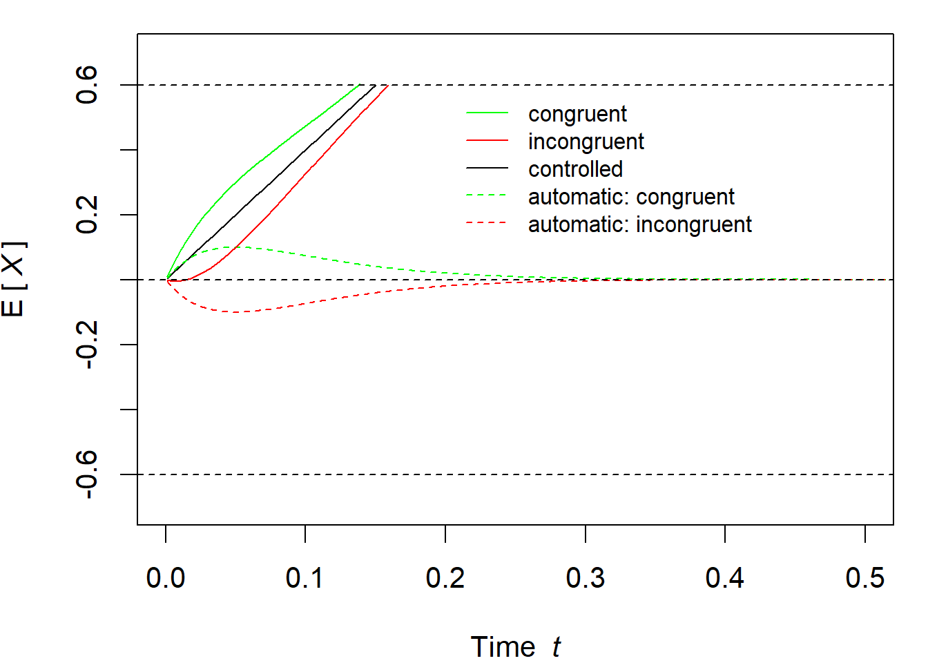

Figure 3.8: Visualization of DMC’s expected time-courses.

As in the standard DDM, a Brownian motion is added to the “final” expected time-course, yielding a fully-fledged diffusion model.

Note that the scaling of parameters in this book deviates from the original DMC publication (Ulrich et al. 2015). The original publication introduced DMC in milliseconds and used a diffusion constant of $\sigma = 4$. In this book, however, we adopt the scaling of dRiftDM, where DDMs are provided with $\sigma = 1$ and in the unit of seconds. Instructions and more details on how to re-scale DMC’s parameters can be found in the vignettes of dRiftDM (see also the Appendix of Koob et al. 2023).

3.2.1.4 Further parameters of DMC

We have already mentioned the boundary $b$, which is typically accuracy-coded in the context of DMC and hence $b$ is a correct and $-b$ is an incorrect response. So far, we have assumed that evidence accumulation starts at $X(0)=0$ (see Figure 3.8). Ulrich et al. (2015) also considered random variability of the starting point to better account for the fast errors often observed in conflict tasks. In principle, the gamma-shaped automatic process already produces a tendency for fast errors, especially for lower values for $\tau$. However, this tendency is not strong enough to fully account for the strong presence of fast errors in conflict task data sets.

The parameter $\alpha$ gives the shape parameters of a Beta distribution stretched to the boundary space $[-b,b]$ from which the starting point is randomly drawn. Note that the exact distribution from which starting values are drawn seems not to affect model predictions much (Ratcliff 2013). Details are provided below in Section 3.2.1.7.

Finally, as in the simple DDM, a non-decision time $t0$ is added to the first-passage times to yield RTs proper. In the original publication, the non-decision time is assumed to follow a normal distribution with mean $t0$ and standard deviation $S_{t0}$. In sum, DMC has eight parameters (plus the diffusion constant $\sigma$):

$b$: boundary
$\mu_c$: drift rate of controlled processing
$t0$: mean of the normally distributed non-decision time
$S_{t0}$: standard deviation of the normally distributed non-decision time
$\alpha$: shape parameter for the starting point Beta distribution
$A$: amplitude of task-irrelevant processing
$\tau$: scale parameter of task-irrelevant processing
$a$: shape parameter of task-irrelevant processing

When fixing the shape parameter $a$ of the task-irrelevant process to $a=2$, then DMC has seven parameters. In general, we recommend fixing $a$ as it leads to more numerically stable predictions.²¹

3.2.1.5 DMC and delta functions

DMC was not developed for one specific conflict task, but rather as a general model accounting for data from various conflict tasks (although the majority of work focus on the Simon and the Eriksen flanker task). Thus, DMC must account for delta functions of different types, and this is indeed one important strength of DMC. In fact, the predicted delta function depends on the peak time of automatic processing. If this peak is early, a negatively-sloped delta function results, if the peak is late, the delta function is positively-sloped instead. This is illustrated in Figure 3.9 for two different amplitudes. As can be seen, the delta functions becomes increasingly positive when $\tau$ increases. Thus, by varying the peak of the automatic activation, DMC can account for various kinds of delta functions.

$Illustration of how the delta function depends on the peak time of the automatic processing, that is, on $\tau$. The amplitude was set to $A=0.1$ and $A=0.15$ in the left and right panel, respectively, and $a=2$ applies in both panels.$

Figure 3.9: Illustration of how the delta function depends on the peak time of the automatic processing, that is, on $\tau$. The amplitude was set to $A=0.1$ and $A=0.15$ in the left and right panel, respectively, and $a=2$ applies in both panels.

3.2.1.6 Summary of DMC

In sum, DMC (Ulrich et al. 2015) translates dual-route models into a DDM by modeling controlled and automatic processing as two separate diffusion processes that are superimposed to yield the overall activation. While controlled processing is conceived as in a standard DDM, the expected time-course of automatic processing first increases and then decreases again back to 0. This form is often referred to as a pulse function and is formally modeled with a rescaled Gamma distribution. By varying the time-point $t$ where this function reaches its maximum, DMC can predict a whole variety of delta functions. The next section provides some advanced mathematical background for those who are interested.

3.2.1.7 Excursus: Details on the Gamma and the Beta distribution

This section is certainly not necessary to understand DMC and to work with this model. However, we provide some details of how DMC’s (rescaled) Gamma and Beta distributions relate to the respective PDFs and their formulas to allow a deeper understanding.

Frst, we begin with the Gamma distribution. In the DMC literature (see also above), the expected time-course of automatic processing is typically formalized with a so-called rescaled Gamma distribution of the form \[\begin{equation} \mathbb{E}[X_a(t)]=A\cdot e^{\left(-\frac{t}{\tau}\right)}\cdot \left[ \frac{t\cdot e}{(a-1)\cdot \tau}\right]^{(a-1)}\,. \tag{3.1} \end{equation}\] In statistics textbooks and also on the internet, you will often find the PDF of the Gamma distribution being described as \[\begin{equation} f(x) = \frac{1}{\Gamma(\alpha)\theta^\alpha}\cdot x^{\alpha-1}\cdot e^{-\frac{x}{\theta}}\quad\text{for }x>0\,, \tag{3.2} \end{equation}\] where $\alpha>0$ and $\theta>0$ are the shape and scale parameter, repectively,²² and $\Gamma$ is the Eulerian Gamma function \[ \Gamma(\alpha) := \int_0^\infty t^{\alpha-1}\cdot e^{-t}dt\,. \] In R, the values of the Gamma distribution as a function of $x>0$ are given by dgamma(x, shape, scale), while the value of the Eulerian Gamma function is given by gamma(x). Let us first rewrite Equation (3.1) whilst omitting the amplitude factor $A$:

\[\begin{equation} \begin{aligned} E[X_a(t)] &= e^{\left(-\frac{t}{\tau}\right)}\cdot \left[ \frac{t\cdot e}{(a-1)\cdot \tau}\right]^{(a-1)}\\ &=\underset{\text{core}}{\underbrace{e^{\left(-\frac{t}{\tau}\right)}\cdot t^{(a-1)}}}\cdot \underset{\text{norming factor}}{\underbrace{\left[ \frac{e}{(a-1)\cdot \tau}\right]^{(a-1)}}}\,. \end{aligned} \tag{3.3} \end{equation}\]

Now compare Equation (3.3) to Equation (3.2) and replace $t$ with $x$, $a$ with $\alpha$, and $\tau$ with $\theta$: The core term is also present in the standard definition in the PDF of a Gamma distribution, but the norming factor differs.

Before we consider the norming factor in more detail, let us determine the mode of $f(x)$. To this end, we take the first derivative of Equation (3.2) and equate it with 0. Because the norming factor does not depend on $x$, we can ignore it and consider the simpler function \[\begin{equation} g(x) = x^{\alpha-1}\cdot e^{-\frac{x}{\theta}}\,. \end{equation}\] The first derivative of $g(x)$ with respect to $x$ is \[\begin{equation} \begin{aligned} \frac{dg(x)}{dx}=g'(x)&= (\alpha-1)\cdot x^{(\alpha-2)}\cdot e^{-\frac{x}{\theta}}-\frac{1}{\theta}x^{(\alpha-1)}\cdot e^{-\frac{x}{\theta}} \\ &= x^{(\alpha-2)}\cdot e^{-\frac{x}{\theta}}\cdot \left[(\alpha-1) - \frac{x}{\theta} \right]\,. \end{aligned} \end{equation}\] We now set $g'(x)=0$ and solve for $x$. Luckily, the first part of $g'(x)$, $x^{(\alpha-2)}\cdot e^{-\frac{x}{\theta}}$, is always larger than 0 if $x>0$, and we can focus on the latter part and solve

\[\begin{align} (\alpha-1) - \frac{x}{\theta} &= 0 \\ (\alpha-1)\cdot\theta &= x \,. \end{align}\]

In terms of Equation (3.1) and (3.3) this means that the function has its maximum at $t_{\text{max}}=(a-1)\cdot\tau$. The final part is now to determine the value Equation (3.1) takes at $t_{\text{max}}$. We again omit the amplitude $A$ first and plug in $t_{\text{max}}$: \[\begin{align} \mathbb{E}[X_a(t_{\text{max}})] &= e^{\left(-\frac{t_{\text{max}}}{\tau}\right)}\cdot \left[ \frac{t_{\text{max}}\cdot e}{(a-1)\cdot \tau}\right]^{(a-1)} \\ &= e^{\left(-\frac{(a-1)\cdot\tau}{\tau}\right)}\cdot \left[ \frac{(a-1)\cdot\tau\cdot e}{(a-1)\cdot \tau}\right]^{(a-1)} \\ &= e^{-(a-1)} \cdot e^{(a-1)} \\ &= 1 \end{align}\] Thus, the function without the factor $A$ has a unity peak and the purpose of the norming factor as used in Equation (3.1) and (3.3) is simply to rescale the Gamma distribution in the way that the maximum is 1. This makes sense, of course, because now multiplying the whole function with $A$ easily allows to vary the amplitude.

Second, we consider the rescaled Beta distribution from which the starting values are drawn. This function is derived as \[\begin{equation} f(x) = \frac{[(x-b_1)\cdot (b_2-x)]^{\alpha-1}}{B(\alpha_1,\alpha_2)\cdot(b_2-b_1)^{2\alpha-1}} \tag{3.4} \end{equation}\] with $\alpha_1=\alpha_2=\alpha$ in our special case and $b_1$ and $b_2$ are the absolute values of the lower and upper end of the distribution. For symmetry, we use $b=b_1=b_2$. $B(\alpha_1,\alpha_2) = B(\alpha,\alpha)$ is the Eulerian Beta function \[ B(\alpha_1,\alpha_2):=\int_0^1 x^{\alpha_1-1}\cdot (1-x)^{\alpha_2-1}dx\,. \] In R, the values of the unscaled Beta distribution as a function of $x\in\{0,\ldots,1\}$ are given by dbeta(x, shape1, shape2), while the value of the Eulerian Beta function is given by beta(shape1, shape2). Several examples of the rescaled Beta distribution as described in Equation (3.4) are visualized in Figure 3.10. As can be seen, with $\alpha=1$, the distribution becomes a uniform distribution.

Figure 3.10: Visualization of several rescaled Beta distributions from which the starting point is randomly drawn in DMC

3.2.2 Shrinking Spotlight model (White et al., 2011)

The Shrinking Spotlight model (SSP) was developed by White, Ratcliff, and Starns (2011) to account for data from Eriksen flanker tasks. An important point for its development is the occurrence of fast errors in the incongruent conditions which suggests that the influence of the flankers is particularly important in the beginning of a trial. Basically, SSP formalizes the zoom lense metaphor of visual attention (B. A. Eriksen and Eriksen 1974) that shrinkens as time increases (C. W. Eriksen and St. James 1986). At the beginning of a trial, attention is wide and the flankers affect processing, but with increasing time, the spotlight becomes more focused and the flanker lose their influence.

3.2.2.1 The Zoom Lense Metaphor as a Shrinking Normal Distribution

Let us assume, as in the experiments by White, Ratcliff, and Starns (2011), that the task of a participant is to respond to the direction of a central arrow (the target). The target is flanked on each side by two flankers. A congruent trial might look like \[< < \hspace{0.2cm}<\hspace{0.2cm} < <\] while \[> > \hspace{0.2cm}<\hspace{0.2cm} > >\] would be an incongruent trial.

Figure 3.11 illustrates an example with an incongruent stimulus display. Each stimulus element is assigned a region of “one unit” (and everything that remains to the left and right is assigned to the outer flankers). A normal distribution is drawn above the display, with its peak located over the target. The vertical dashed lines mark the boundaries of the regions for each stimulus element, and the area of these regions under the normal distribution is considered the amount of visual attention allocated to each stimulus element. To better illustrate this, the portion corresponding to the target is shaded in gray. The target’s region extends from –0.5 to 0.5, the right inner flanker’s region from 0.5 to 1.5, and the right outer flanker’s region from 1.5 to $+\infty$.

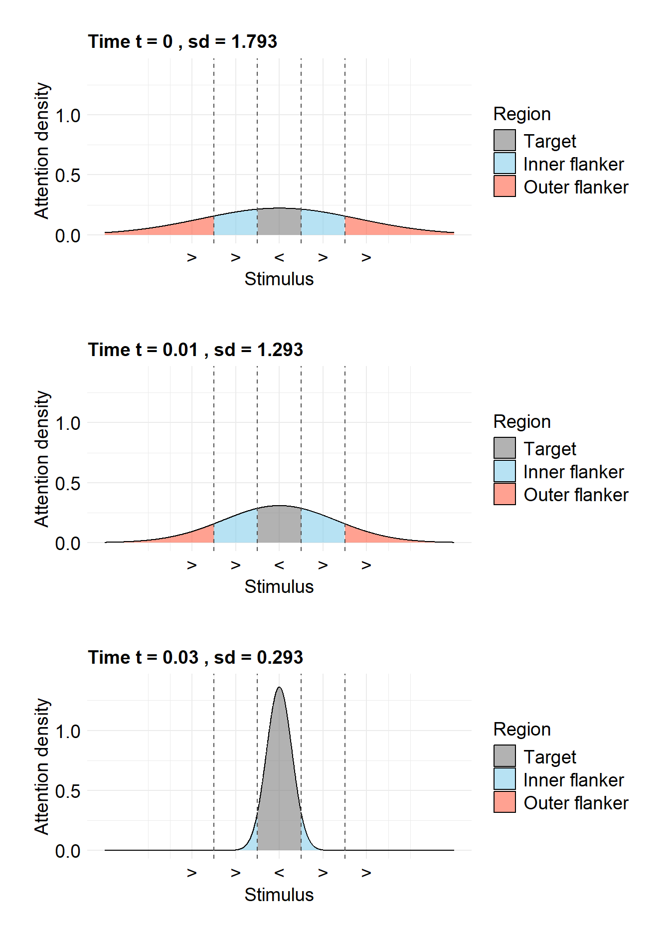
Illustration of the Shrinking Spotlight model (White et al. 2011): The normal distribution centered above the target becomes narrower with increasing time in a trial, that is, its standard deviation becomes smaller. Consequently, the area above the target (in gray) becomes larger and that above the flankers becomes smaller.

Figure 3.11: Illustration of the Shrinking Spotlight model (White et al. 2011): The normal distribution centered above the target becomes narrower with increasing time in a trial, that is, its standard deviation becomes smaller. Consequently, the area above the target (in gray) becomes larger and that above the flankers becomes smaller.

3.2.2.2 Formalizing the Amount of Attention to the Target and the Flankers

The “narrowing” of the spotlight is now modeled by the standard deviation $\sigma_a$ of the normal distribution becoming progressively smaller (see the three parts of Figure 3.11). With each time step $t$, the standard deviation decreases linearly by a fixed amount $r_d$, until it reaches a minimum value of $\sigma_{\text{min}}=0.001$.

If we take the initial value of the standard deviation as $\sigma_a(0)=1.793$ (see Table 2 in White, Ratcliff, and Starns 2011), then the standard deviation is calculated as \[ \sigma_a(t)=\text{max}(1.793-r_d \cdot t\hspace{0.2cm},\hspace{0.2cm}0.001)\,. \] Using this, we can now further calculate the proportion of the area over the target ($a_T$), the (right) inner flanker ($a_I$), and the (right) outer flanker ($a_O$). If $\Phi$ is the PDF of a normal distribution, then we obtain the desired area proportions as \[ a_T = \int_{-0.5}^{0.5}\Phi(0,sd_a(t))dt\hspace{0.7cm} a_I = \int_{0.5}^{1.5}\Phi(0,sd_a(t))dt\hspace{0.7cm} a_O = \int_{1.5}^{\infty}\Phi(0,sd_a(t))dt \,. \] These values are then multiplied by the parameter $p$ (“perceptual input”), whose sign depends on the direction of the respective arrow. The total drift rate at time $t$, that is, $\mu(t)$, results from the sum of the products of the individual attention values $a_i$ and their respective perceptual inputs $p_i$. Since both flankers appear twice, their values must be multiplied by 2, thus \[ \mu(t)=2\cdot p_O\cdot a_O(t) + 2\cdot p_I\cdot a_I(t) + p_T\cdot a_T(t)\,. \]

3.2.2.3 Expected Time-Course and Drift Rate

How do the drift rates and the respective expected time-course look like for SSP? Figure 3.12 conceptually replicates Figure 6 in White, Ratcliff, and Starns (2011) with the drift rates for congruent and incongruent trials in the left panel and the respective expected time-courses in the right panel.²³ First, as one can see, the drift rate $\mu(t)$ is actually time-independent in congruent trials. This makes sense, of course, as the target and the flankers all promote the same response, just with different proportions as time increases. Second, however, $\mu(t)$ does depend on time $t$ for incongruent trials. Initially, the flankers drive the activation toward the wrong response and the drift rate is negative, but they become less and less influential until the target dominates evidence accumulation and the positive drift rate drives the process toward the correct response.

Figure 3.12: Drift Rate (left) and expected time-course of activation (right) at each time-point $t$.

3.2.2.4 Further Parameters of SSP and Summary

The boundary $b$ is typically accuracy-coded in the context of SSP. The parameter $p$ represents the perceptual input, the parameter $\sigma_0$ the initial standard deviation of the normal distribution at $t=0$, and the parameter $r$ the rate of its decline. Finally, a non-decision time $t0$ is added to the first-passage times. In sum, SSP has at least 5 parameters (plus the diffusion constant $\sigma$):

$b$: boundary
$t0$: mean of the non-decision time
$p$: perceptual input
$\sigma_0$: standard deviation of the normal distribution at $t=0$
$r$: rate of decline for the standard deviation of the normal distribution

Just like any other DDM, SSP has also been extended with trial-by-trial variability in non-decision time, starting point, or drift rate (White, Ratcliff, and Starns 2011). For example, one might assume the non-decision time to result from a uniform distribution with mean $t0$ and range $S_{t0}$

3.2.3 Exercise: Delta Function Predictions for DMC and SSP

We introduced DMC and SSP as examples of cognitive models for conflict tasks. Both models are prebuilt in dRiftDM, however, and are thus easy to use. To work with DMC or SSP, one simply creates a corresponding object from the functions dmc_dm() or ssp_dm(), respectively.

The following code shows how to create DMC with the additional parameters $S_{t0}$ (the standard deviation of the non-decision time) and $\alpha$ (the shape parameter of the Beta distribution from which the variable starting point is drawn):

myDMC <- dmc_dm(var_start = TRUE, var_non_dec = TRUE)

The model is, of course, a bit more complicated as compared to a standard DDM:

print(myDMC)

## Class(es): dmc_dm, drift_dm
## 
## Current Parameter Matrix:
##        muc   b non_dec sd_non_dec  tau a    A alpha
## comp     4 0.6     0.3       0.02 0.04 2  0.1     4
## incomp   4 0.6     0.3       0.02 0.04 2 -0.1     4
## 
## Unique Parameters:
##        muc b non_dec sd_non_dec tau a A alpha
## comp   1   2 3       4          5   0 6 7    
## incomp 1   2 3       4          5   0 d 7    
## 
## Special Dependencies:
## A ~ incomp == -(A ~ comp)
## 
## Custom Parameters:
##        peak_l
## comp     0.04
## incomp   0.04
## 
## Deriving PDFs:
##   solver: kfe
##   values: sigma=1, t_max=3, dt=0.001, dx=0.001, nt=3000, nx=2000
## 
## Observed Data: NULL

If we were just interested in the parameters and want to change them, this again could be done in the standard way:

coef(myDMC) # Show parameters

##        muc          b    non_dec sd_non_dec        tau          A      alpha 
##       4.00       0.60       0.30       0.02       0.04       0.10       4.00

coef(myDMC)["A"] <- 0.2 # Change parameter A

Creating and interacting with SSP works similarly:

mySSP <- ssp_dm()
coef(mySSP)

##             b       non_dec range_non_dec             p          sd_0 
##          0.60          0.30          0.05          3.30          1.20

Now it is your turn to explore DMC and SSP with dRiftDM:

1.) Create DMC and explore the model predictions a bit. In particular, explore how the delta function depends on the parameters $\tau$ and $A$.

2.) Compare DMC with and without starting point variability. Can DMC account for the typical results without starting point variability?

3.) Create SSP and explore the model predictions, in particular the shape of the delta function. Could SSP somehow account for Simon data as well?

4.) Look at the CAF predicted by SSP. Why does SSP account for fast errors even without starting point variability?

3.3 Exercise Solutions:

3.3.1 Solutions for the Exercise on the Ratcliff DDM

There is no general solution. However, the following code snippets and summaries will help you to check if you were able to achieve the main goals for each exercise.

The following code shows how to create and modify the Ratcliff DDM with all sources of parameter variability and how to subsequently plot the quantiles and the CAF. To speed up the generation of the model predictions, we slightly increased dx and dt:

# get the model and modify the parameter values
my_model <- ratcliff_dm(
  var_non_dec = TRUE, var_start = TRUE, var_drift = TRUE,
  dx = .005, dt = .005
)
coef(my_model) <- c(
  muc = 4, b = 0.5, non_dec = 0.2, range_non_dec = 0.1,
  range_start = 1, sd_muc = 1.2
)

# plot the quantiles and the CAF side-by-side
par(mfrow = c(1, 2), cex = 1.0)
plot(
  calc_stats(my_model, type = c("quantiles", "cafs"))
)

When experimenting with the model, you might arrive at the conclusion that typical parameter ranges in the context of experimental psychology are approximately as follows:

$\mu_c \in \{1, \dots, 7\}$
$b \in \{0.3, \dots, 1.0\}$
$t0 \in \{0.2, \dots, 0.7\}$
$s_{t0} \in \{0, \dots, 0.25\}$
$s_{z} \in \{0, \dots, 1.5\}$
$s_{\mu_c} \in \{0, \dots, 2\}$

A custom plot of the model’s predicted PDFs can be generated like this:

# Get the pdfs and extract the respective vectors as well as the time space 
pdf_list <- pdfs(my_model)
pdf_corr <- pdf_list$pdfs$null$pdf_u
pdf_err <- pdf_list$pdfs$null$pdf_l
t_vec <- pdf_list$t_vec

# Plot everything
par(mfrow = c(1, 2), cex = 1.0)
plot(pdf_corr ~ t_vec,
  ylab = "f(RT)", xlab = "Time [s]", type = "l",
  xlim = c(0, 1)
)
plot(pdf_err ~ t_vec,
  ylab = "f(RT)", xlab = "Time [s]", type = "l",
  xlim = c(0, 1)
)

The following code shows how to create a delta function for the Ratcliff DDM with the two conditions comp and incomp. The parameter values were chosen in a way that incompatible trials have a smaller drift rate, a higher boundary, and a longer non-decision time:

# Create the model
my_model <- ratcliff_dm()
conds(my_model) <- c("comp", "incomp")

## resetting parameter specifications

my_model <- modify_flex_prms(
  my_model,
  instr = " ~ "
)

# Set some reasonable parameter values
coef(my_model)

##       muc.comp     muc.incomp         b.comp       b.incomp   non_dec.comp 
##            3.0            3.0            0.6            0.6            0.3 
## non_dec.incomp 
##            0.3

coef(my_model)[c(2,4,6)] <- c(2.5, 0.7, 0.4)
par(mar = c(4,4,1,1), cex = 1.3)
plot(
  calc_stats(
    my_model, type = "delta_funs", minuends = "incomp", subtrahends = "comp"
  ), ylim = c(0, 0.5)
)

When trying out different parameter values you should notice that the Ratcliff DDM has a hard time to predict negatively-sloped delta functions with reasonable parameter settings, especially those that initially increase and then decrease. For those kind of delta functions, we need DMC (see Section 3.2.1).

3.3.2 Solutions for the Exercise on SSP and DMC

There is again no general solution, but we’ll provide code snippets and a short summary.

The following code shows how to create and modify DMC with respect to $A$ and $\tau$, and how to subsequently plot the predicted delta function.

my_model <- dmc_dm()
coef(my_model)[c("A", "tau")] <- c(0.2, 0.12)
par(mar = c(4,4,1,1), cex = 1.3)
plot(
  calc_stats(
    my_model, type = "delta_funs", minuends = "incomp", subtrahends = "comp"
  )
)

When experimenting with $A$ and $\tau$, you should arrive at the conclusion that…

the general level (i.e., the vertical distance relative to zero) of the delta function increases, the larger $A$.
the slope of the delta function increases the larger $\tau$. If $\tau$ is small, the delta function is decreasing (i.e., negatively-sloped). If $\tau$ is large, the delta function is increasing (i.e., positively-sloped).

the typical results in conflict tasks are delta functions that are either decreasing (Simon task) or at least decrease at the largest quantile levels (i.e., for slow responses: Flanker task). Additionally, we almost always observe fast errors in incompatible trials. Let’s see if DMC can account for both without assuming trial-by-trial variability in the starting point.

dmc_start_var <- dmc_dm(var_start = TRUE) # this is also the default
dmc_no_start_var <- dmc_dm(var_start = FALSE)


par(mfrow = c(1,2), cex = 1.0)
# Plot CAFS and the delta function for the model WITH start point variability
plot(
  calc_stats(
    dmc_start_var, type = c("cafs", "delta_funs"), 
    minuends = "incomp", subtrahends = "comp"
  )
)

# Plot CAFS and the delta function for the model WITHOUT start point variability
plot(
  calc_stats(
    dmc_no_start_var, type = c("cafs", "delta_funs"), 
    minuends = "incomp", subtrahends = "comp"
  )
)

Apparently, DMC can predict the typical results from conflict tasks with and without variability in the starting point. However, especially fast errors are way less pronounced without it.

The following code shows how to create and modify SSP with respect to $p$ and $sd_0$, and how to subsequently plot the predicted delta function.

my_model <- ssp_dm()
coef(my_model)[c("p", "sd_0")] <- c(4, 0.5)

par(mar = c(4,4,1,1), cex = 1.3)
plot(
  calc_stats(
    my_model,
    type = "delta_funs", minuends = "incomp", subtrahends = "comp"
  )
)

When experimenting with the SSP, you should find that it can reproduce the positively sloped delta function typically observed in the flanker task. However, the SSP cannot account for the negatively-sloped delta function commonly found in the Simon task (at least not with reasonable parameter values).

The following code shows how to create SSP without trial-by-trial variability in the starting point, and how to subsequently plot the predicted CAF.

my_model <- ssp_dm(var_start = FALSE) # actually the default

par(mar = c(4,4,1,1), cex = 1.3)
plot(
  calc_stats(my_model, type = "cafs")
)

As is evident, SSP naturally predicts fast errors in incompatible trials. The reason for this is that the influence of the flankers is initially large, but then fades as attention narrows down on the target. Consequently, the decision is prone for selecting the wrong response in incompatible trials early in the trial, but not later in the trial, and this implies fast errors.

It is also known as the simple DDM or standard DDM.↩︎
This is not too much surprising if we remember that a RW turns into a DDM in the limit.↩︎
This is sometimes called a response coding↩︎
Note that we have already implicitly covered a bias in the starting point and even trial-by-trial variability in the Exercise in Section 2.2.3.5 ↩︎
Note that a fixed value for $z$, $\mu$, and $t0$ as in the simplest DDM is only a special case when assuming each $s_{z}$, $s_{\mu}$, and $s_{t0}$ to be zero.↩︎
Time-dependent boundaries are covered in Chapter 5. Implementing a time-dependent diffusion parameter is currently not supported in dRiftDM, primarily because this case is extremely rare.↩︎
The technical reason is that the derivative of the general equation of the rescaled Gamma distribution function is undefined at $t=0$, which introduces an initial numerical error that becomes apparent as the diffusion process progresses over time.↩︎
There is also an alternative parametrization with a rate parameter $\lambda = \frac{1}{\theta}$.↩︎
Conceptual, because White, Ratcliff, and Starns (2011) plot the sum of the drift rates while we plot the expected time-course of the evidence accumulation process (taking the step size in the unit of seconds into account).↩︎