2 Mathematical Background

This chapter may be somewhat inconvenient for those new to understanding and using DDMS. However, gaining a solid background of stochastic processes, Markov chains, and random walks (RWs) is essential on the path to a “real” DDM. By the end of this chapter, you will be much better equipped to engage with the terminology and concepts commonly encountered in this context.

Extensive and in-depth treatments of RWs and diffusion processes are given in, for example, Cox and Miller (1965) or Schwarz (2022). We here present information tailored the purposes of this book, which is also covered in much more detail in an article by Diederich and Busemeyer (2003) and a book chapter by Diederich and Mallahi-Karai (2018).

We begin with a brief introduction to the core ideas of stochastic processes and Markov chains, followed by a more detailed treatment of RWs. Only then do we turn to DDMs, and you will see that they are, in fact, a kind of RW. In that section, we also treat other aspects, such as dealing with the durations of perceptual and motor processes in a DDM, to give a bit more intuition about how dRiftDM works internally.

2.1 Stochastic Processes and Markov Chains

Stochastic processes are the mathematics underlying sequential sampling models, of which RWs and DDMs are examples. In our context, a stochastic process is a collection of random variables \[ \{{X}_t\}_{t\in T} \] that take values of a set \(S\), the state space, which can be discrete or continuous. The index set \(T\) is referred to as the time space in our context and may also either be discrete or continuous. Basically, then, a stochastic process develops over time and takes different values of \(S\). It does so with uncertainty, that is, in a stochastic way, and at each time-point (or index) \(t\), the state depends only on the state at time-point \(t-1\), but not on how the state at \(t-1\) was reached. We will first consider the simplest case with \(T\) and \(S\) being discrete, that is \(t\in\mathbb{N}_0\) and \({X}_t\in\mathbb{Z}\). Such a process is also known as a Markov chain.

Let us first look at a very simple example about weather forecasting and introduce some concepts we will encounter later again. For simplicity, the weather is either sunny (\(S\)) or rainy (\(R\)). The random variables \({X}_0, {X}_1, {X}_2, \ldots\) take either the value \(S\) or \(R\) and represent the weather over time. If we further assume that tomorrow’s weather depends only on today’s weather, then we add the Markov property. In that case, we can describe the weather development with a transition matrix \(P\), for example,

\[ P= \begin{matrix}t \end{matrix} \begin{matrix} \scriptstyle S \\ \scriptstyle R\end{matrix} \overset{\phantom{kk}t+1 \\ \scriptstyle S \phantom{klkkk} R}{\begin{bmatrix} 0.7 & 0.3 \\ 0.2 & 0.8 \end{bmatrix}}\,. \]

In this matrix, the rows represent the current state at day \(t\), that is, were the process “comes from”, and the columns represent the state at day \(t+1\), that is, where the process will go to. The first row and column represent a sunny day, while the second row and column represent a rainy day. This means that if it is sunny today, it will be sunny again tomorrow with probability \(p=0.7\) (the process remains in the same state), and rainy with probability \(p=0.3\) (the process switches to a different state). Likewise, if it is raining today, it will be rainy tomorrow with probability \(p=0.8\), but sunny with probability \(p=0.2\). More formally, each entry of \(P\) defines a transition probability, namely \[ p_{ij}=p(X_{t+1}=j|X_{t}=i)\,. \] The matrix is called a stochastic matrix if all entries are non-negative and the entries within each row add to 1.

Simulating the development of this stochastic process is straightforward. We simply specify an initial state, and from there, the process evolves according to the transition matrix \(P\):

states <- c("S", "R") # Define the possible states
howManyDays <- 10 # How many days we want to trace?

P <- matrix(
  c(
    0.7, 0.3, # Create the transition matrix
    0.2, 0.8
  ),
  nrow = 2,
  byrow = TRUE
)

current_state <- 1 # Initial state (1 = S, 2 = R)

set.seed(123) # For reproducibility
weather <- character(howManyDays) # Prepare container

# Then we simulate the days beginning with the initial state
for (i in 1:howManyDays) {
  weather[i] <- states[current_state] # Current weather
  current_state <- sample( # Next day's weather
    x = c(1, 2),
    size = 1,
    prob = P[current_state, ]
  )
}

print(weather)

##  [1] "S" "S" "R" "R" "S" "R" "R" "R" "S" "S"

More details and examples for specific Markov chains are provided in Diederich and Mallahi-Karai (2018). We will now consider RWs, the Markov chain of most interest to our purposes.

2.2 Random Walks

Remember from Section 1.2 that response selection is often conceived as the accumulation of evidence over time \(t\) with some random fluctuations. A RW is the most fundamental Markov chain that fulfills these criteria and, in fact, underlies many more sophisticated models, such as the DDM. We will therefore cover and explain some general concepts related to RWs in considerable detail.

In the following sections, the state space is \(S=\mathbb{Z}\) and the time space is \(T=\mathbb{N}_0\). In other words, the differences between each time-step are \(\Delta t=1\) and in each state, the differences are \(\Delta x=1\). This notion will become important later.

2.2.1 Simple, Symmetric Random Walk

2.2.1.1 The Concept

The simplest case is the symmetric RW with unrestricted evolution. At each time-point \(i\in T\), a random variable \({Y}\) is realized with the probability mass function \[\begin{align} P({Y}_i = 1) = P({Y}_i = -1) = 0.5\,. \end{align}\] All such (Bernoulli-distributed) random variables are conceived as mutually independent. The position of the RW in the state space at \(t\) is then the sum of the \(Y_t\) \[\begin{equation} {X}_t = \sum_{i=1}^t{Y}_i\text{ with } {X}_0=0\,, \end{equation}\] or, put differently, \[\begin{equation} {X}_{t+1} = {X}_{t}+{Y}_{t}\,. \tag{2.1} \end{equation}\]

This last form is an example of a stochastic difference equation. As all random variables \(Y\) are independent from each other, \({Y}_{t}\) is also independent from \({X}_{t}\), and the Markovian property is fulfilled. In other words, the distribution of \({X}_{t+1}\) only depends on \({X}_{t}\), but not on how this position at \(t\) was reached (see also Schwarz 2022).

The evolution of this RW can easily be simulated (in more or less elegant ways). In the present case, it suffices to sample a large number of realizations of \({Y}_t\) and then consider their cumulative sum. Figure 2.1 visualizes a typical run of the following code.

par(mar = c(4, 4, 1, 1), cex = 1.3)


T_max <- 50 # Maximum time T
p <- 0.5 # Probability of moving up (+1)
X_0 <- 0 # Initial condition at t = 0

t <- c(0:T_max)
set.seed(1) # For reproducibility

X_t <- cumsum(sample(
  x = c(1, -1), # Realize the X_t
  size = T_max,
  prob = c(p, 1 - p),
  replace = TRUE
))
X_t <- c(X_0, X_t) # Add initial condition

plot(X_t ~ t,
  type = "l",
  ylim = c(-8, 8),
  xlab = expression(plain("Time ") ~ italic(t)),
  ylab = expression(italic(X)[italic(t)]),
  main = "Simple, symmetric Random Walk",
  cex.main = 0.8
)
abline(h = c(-10:10), lty = 3, col = "gray80")
abline(v = c(0:T_max), lty = 3, col = "gray80")

Figure 2.1: Visualization of a simple, symmetric Random Walk with 50 time-steps.

2.2.1.2 Expected Value and Variance

Now imagine we would simulate not one but an infinite number of such RWs and calculate the mean and the variance of \({X}_t\) at each \(t\). This would be the expected value and the variance of the respective stochastic process at time \(t\). Calculating them is a typical question when analyzing stochastic processes and is fairly easy in this case, despite its stochastic component.⁴

• The expected value of each \({X}_t\) is straightforward. Because \(P({Y}_i = 1) = P({Y}_i = -1) = 0.5\), it follows \(\mathbb{E}({Y}_i) = 0.5\cdot 1 + 0.5\cdot -1 = 0\). As \({X}_t\) is the sum of all \({Y_i}\) up to time-point \(t\), it follows \[\mathbb{E}({X}_t) = 0\,.\]
• We now calculate first the variance of \({Y}_i\) as \[\begin{align*} V({Y}_i) &= \mathbb{E}[({Y}_i-\mathbb{E}({Y}_i))^2] \\ &= (-1 - 0)^2\cdot 0.5+(1-0)^2\cdot 0.5 \\ &= 1\,. \end{align*}\] The variance of \({X}_t\) can be obtained by taking the variance of the sum of the random variables \({Y}_i\). As all \(Y_i\) all assumed independent of each other, this sum breaks down to \[\begin{align*} V({X}_t) &= \sum_{i = 1}^t V({Y}_i) \\ &= \sum_{i = 1}^t 1 \\ &= t\,. \end{align*}\]

2.2.2 Random Walk with Drift

2.2.2.1 The Concept

Now consider a typical 2-AFC task. The participant (or their cognitive system) extracts evidence (or activation) from the presented stimulus, and we assume that the random variable \({X}_t\), evolving over time, represents this evidence for each time-point \(t\). The RW covered in the previous paragraph does not help much for now, as it meanders around zero (remember that its expected value was zero) and seems not to represent systematic evidence for either of the two stimuli or responses associated with them.

We thus extend the RW by allowing the random variables \({Y}_i\) to take their values with arbitrary probabilities \(p\) and \(1-p\), that is, \[\begin{align} P({Y}_i = 1) = p\quad\text{und}\quad P({Y}_i = -1) = 1-p\,. \end{align}\] Accordingly, with \(p > 0.5\), each step is more likely to yield a value of 1 than -1, and thus the chance that \({X}_t\) is positive is higher than the chance that it is negative. In a psychological context, we can interpret a positive value as evidence in favor of one stimulus. If \(p < 0.5\), \({X}_t\) is more likely to become negative, which counts as evidence for the other stimulus. Both possibilities are visualized in Figure 2.2. In the left panel, processes tend toward the upper area of the plot, while in the right panel, they tend toward the lower area.

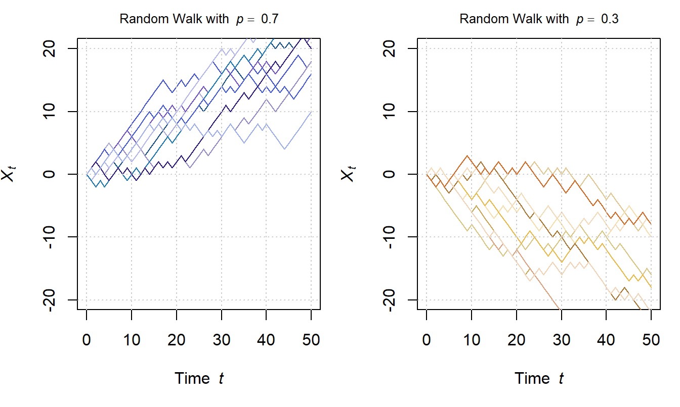
Figure 2.2: Visualization of Random Walks with 50 time-steps and \(p=0.7\) (left panel) versus \(p=0.3\) (right panel).

2.2.2.2 Expected Value and Variance

Let us again calculate the expected value and the variance of \({X}_t\).

• The expected value of each \({Y}_i\) is now \[\begin{align*} \mathbb{E}({Y}_i) &= 1 \cdot p + (-1)\cdot (1-p) \\ &= p -1 + p\\ &= 2 p -1\,. \end{align*}\] As again, \({X}_t\) is the sum of the random variables \({Y}_i\), it follows \[\begin{align*} \mathbb{E}({X}_t) &= \mathbb{E}\left( \sum_{i=1}^t {Y}_i \right) \\ &= \sum_{i=1}^t \mathbb{E}({Y}_i) \\ &= t (2 p-1)\,. \end{align*}\]
• Calculating the variance of \({Y}_i\) takes a bit more of writing, but is not too complicated: \[\begin{align*} V({Y}_i) &= \mathbb{E}[({Y}_i-\mathbb{E}({Y}_i))^2] \\ &= (1-[2p-1])^2\cdot p + (-1-[2p-1])^2\cdot (1-p) \\ &= (1-2p+1)^2\cdot p + (-1-2p+1)^2\cdot (1-p) \\ &= (2-2p)^2\cdot p + (2p)^2\cdot(1-p) \\ &= (4-8p+4p^2)\cdot p + 4p^2\cdot (1-p) \\ &= 4p-8p^2+4p^3+4p^2-4p^3 \\ &= 4p - 4p^2 \\ &= 4p(1-p)\,. \end{align*}\] The variance of \({X}_t\) is again the sum of the variances of the independent random variables \({Y}_i\), that is, \[\begin{align*} V({X}_t) &= \sum_{i = 1}^t V({Y}_i) \\ &= \sum_{i = 1}^t 4p(1-p)\\ &= 4pt(1-p)\,. \end{align*}\]

2.2.2.3 Excursus: Occupation Probabilities and Forward and Backward Equations

The content of this section is not essential for understanding the subsequent material and can safely be skipped. However, it may help you get used to thinking in terms of RWs. Eventually, we will introduce the concepts of forward and backward equations in a simple setting (see also Schwarz 2022 for more information) and similar concepts are mentioned at a later point again.

So far, we have considered the start of any RW to be at \((0,0)\). That is, at \(t=0\), we assumed \({\bf X}_t = 0\). We now relax this and consider the starting point as an additional variable \(k\).

An important quantity of interest is the probability \[P(k,m,n)\] which is the probability that a RW starting at state \(k\) takes state \(m\) (\(k,m\in\ S\)) after exactly \(n\) time-steps. In other words, the probability that a RW starts at \((0,k)\) and terminates at \((n,m)\). We will denote this in the following with \((0,k)\rightarrow(n,m)\). Note that, if we treat \(m\) as a variable, this would give us the probability mass function about the possible states of a RW starting at \(k\) after \(n\) time-steps. Because the RW must have a state at this time-step, they would all sum up to 1, \[ \sum_{m\in S} P(m;k,n)=1\,. \]

Of course, there are some easy special cases. For example, if \(n=0\) and \(k=m\) then \(P(k=m,m,n=0)=1\). This means that the probability of starting at \(m\) and ending in \(m\) after exactly \(n=0\) steps is one. Further, if \(n=1\), the two probabilities that can occur are \(P(k,m=k+1,n=1)=p\) and \(P(k,m=k-1,n=1)=1-p\). This simply means that after one step, the process either went up with probability \(p\) or down with probability \(1-p\).

Now let us have a look at the more interesting cases and learn about a general principle about how \(P\) can be determined. We distinguish two cases, the first leads us to the forward equation, the second to the backward equation, but both will give us the same solution. In either case, we split the whole set of possible RWs into two subsets, by conditioning on either the direction of the first or last step of the whole RW.

First, we consider how to condition on the last step (see Fig. 2.3, left panel). The target \((n,m)\) can be reached in exactly two ways from the state taken at time-point \(n-1\). More precisely, the last step can be

• \((n-1,m+1)\rightarrow(n,m)\) with probability \(1-p\) (a “downward” step), or
• \((n-1,m-1)\rightarrow(n,m)\) with probability \(p\) (an “upward” step).

What are the probabilities of being at state \(m+1\) or \(m-1\) at time-point \(n-1\), that is, right before the final step? By our definition this probability is

• \(P(k, m+1, n-1)\) when we ended up at \((n-1,m+1)\), and
• \(P(k, m-1, n-1)\) when we ended up at \((n-1,m-1)\).

Given the independence of the random variables \({Y}_i\) and the Markovian property, the overall probability of ending at \((n,m)\) when coming from \((n-1,m-1)\) is \[P(k, m-1, n-1)\cdot p\] and that of ending at \((n,m)\) when coming from \((n-1,m+1)\) is \[P(k, m+1, n-1)\cdot (1-p)\,.\] As both possible ways of reaching \((n,m)\) are mutually exclusive, the probability of ending in \((n,m)\) is their sum, that is \[\begin{equation} P(k,m,n)=\underset{\text{final step up}}{\underbrace{P(k, m-1, n-1)\cdot p}} + \underset{\text{final step down}}{\underbrace{P(k, m+1, n-1)\cdot (1-p)}}\,. \tag{2.2} \end{equation}\]

This, however, is only one way to condition on. As an alternative, we now consider how to condition on the first step (see Fig. 2.3, right panel). The first step can take exactly two ways and end in exactly two states at \(n=1\). More precisely, the first step can be

• \((0,k)\rightarrow(1,k-1)\) with probability \(1-p\) (a “downward” step), or
• \((0,k)\rightarrow(1,k+1)\) with probability \(p\) (an “upward” step).

Following this first step, we are left with \(n-1\) steps to reach the target \((n,m)\) from either \((1,k-1)\) or \((1,k+1)\). The probability of doing so is by definition

• \(P(k+1, m, n-1)\) when the first step ended at \((1,k+1)\), and
• \(P(k-1, m, n-1)\) when the first step ended at \((1,k-1)\).

As the two possibilities for the first step are again mutually exclusive, it follows \[\begin{equation} P(k,m,n)=\underset{\text{first step up}}{\underbrace{P(k+1, m, n-1)\cdot p}} + \underset{\text{first step down}}{\underbrace{P(k-1, m, n-1)\cdot (1-p)}}\,. \tag{2.3} \end{equation}\]

What is achieved by doing so? By conditioning on either the last step or the first step, both Equation (2.2) and (2.3) reduce the problem to-be-solved in \(n\) steps into one of only involving \(n-1\) steps. However, they slightly differ in how they do this and which of the three variables is held constant. First, in Equation (2.2), the (start) state \(k\) at \(n=0\) is fixed and \(P(k,m,n)\) is determined from this state on. Hence, the resulting equation is called forward equation \(f\) and can be simplified to \[\begin{equation} f_k(m,n)=f_k(m-1,n-1)\cdot p + f_k(m+1,n-1)\cdot (1-p)\,. \tag{2.4} \end{equation}\] Second, in Equation (2.3), the (end) state \(m\) at \(n\) is fixed and \(P(k,m,n)\) is determined from this state. Hence, the resulting equation is called backward equation \(b\) and can be simplified to \[\begin{equation} b_m(k,n)=b_m(k+1,n-1)\cdot p + b_m(k-1,n-1)\cdot (1-p)\,. \tag{2.5} \end{equation}\] With initial state \(f_k(m=k,n=0)=b_m(k=m,n=0)=1\) and otherwise \(f_k=b_m=0\), the forward and the backward equation can be used in a recursive way to calculate \(P(k,m,n)\).

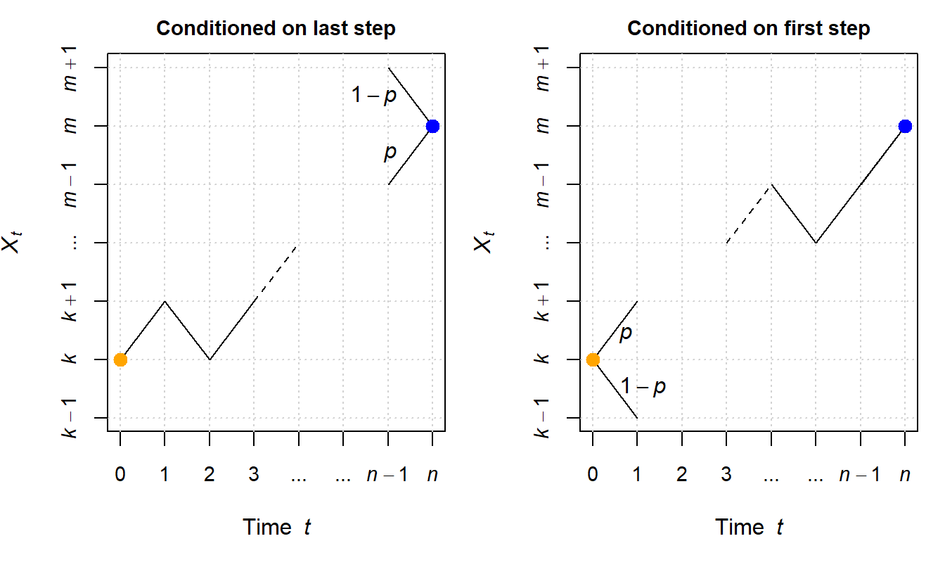
Figure 2.3: Illustration of how Random Walks from \((0,k)\) (orange dot) to \((t,m)\) (blue dot) are conditioned either on the last step (left panel) or on the first step (right). Conditioning on the last step yields the forward equation, and conditioning on the first step yields the backward equation.

Implementing the forward and backward equations in R is not very difficult once we understand their recursive nature. Basically, the following code is taken directly from Equations (2.2) and (2.3). Additionally, we must stop the recursion if \(n=0\), that is, if the equation has called itself sufficiently often.⁵

forward <- function(k, m, n, p) {
  # time = 0
  if (n == 0) {
    return(ifelse(k == m, 1, 0))
  }
  # recursion
  res <- forward(k, m - 1, n - 1, p) * p + forward(k, m + 1, n - 1, p) * (1 - p)
  return(res)
}

backward <- function(k, m, n, p) {
  # time = 0
  if (n == 0) {
    return(ifelse(k == m, 1, 0))
  }
  # recursion
  res <- backward(k + 1, m, n - 1, p) * p + backward(k - 1, m, n - 1, p) * (1 - p)
  return(res)
}

If we now want to determine the probability of being in state \(m=16\) in \(n=10\) time-steps when starting at state \(k=12\) with the probability of moving up \(p=0.6\), we could use either function, giving us the same value for \(P(k=12, m=16, n=10)\):

k <- 12 # Start state
m <- 16 # Target state
n <- 10 # Steps
p <- 0.6 # Probability of moving one step up

forward(k, m, n, p)

## [1] 0.2149908

backward(k, m, n, p)

## [1] 0.2149908

Despite the instructive derivation of the forward and backward equation, the probability \(P(k,m,n)\) can also be calculated using the binomial distribution in our current simple case (see, e.g., Schwarz 2022). What we need to determine is how many steps upwards and downwards are required to match the displacement \(m-k\). Let \(x\) and \(y\) be the numbers of up- (+1) and downward (-1) steps. Their sum must, of course, match the whole number of steps, that is, \[x+y=n\,.\] In addition, the overall displacement during the \(n\) steps must be equal to the difference in \(x\) and \(y\), \[ m-k=x-y\,. \] From these equations, we can calculate \(x\) and \(y\). First we rearrange \(x+y=n\) slightly to \[ x=n-y\quad\text{and}\quad y=n-x \] and plug these into the second equation. We first determine \(x\) as \[\begin{equation} \begin{aligned} m-k&=x-y\\ \Leftrightarrow m-k&=x-(n-x)\\ \Leftrightarrow m-k&=2x-n\\ \Leftrightarrow m-k+n&=2x\\ \Leftrightarrow \frac{m-k+n}{2}&=\boxed{x=\frac{n+m-k}{2}}\,. \end{aligned} \end{equation}\] We can similarly determine \(y\) as \[\begin{equation} \begin{aligned} m-k&=x-y\\ \Leftrightarrow m-k&=n-y-y \\ \Leftrightarrow m-k&=n-2y \\ \Leftrightarrow m-k-n&=-2y \\ \Leftrightarrow \frac{m-k-n}{2}&=-y\\ \Leftrightarrow \frac{-m+k+n}{2}&=\boxed{y=\frac{n-m+k}{2}}\,.\\ \end{aligned} \end{equation}\]

k <- 12 # Start state
m <- 16 # Target state
n <- 10 # Steps
p <- 0.6 # Probability of moving one step up

x <- (n + m - k) / 2
y <- (n - m + k) / 2
print(paste0(x, " steps up, and ", y, " steps down"))

## [1] "7 steps up, and 3 steps down"

Thus, for one particular sequence of up- and downward movements, we reach the displacement \((0,k)\rightarrow (n,m)\) with a probability of \[ p^x\cdot (1-p)^y\,. \] As further the order of up- and downward movements is arbitrary, we multiply this probability with the binomial coefficient \(\binom{x+y}{x}\) and get \[ P(k,m,n)=\binom{x+y}{x}\cdot p^x\cdot (1-p)^y\,. \] To calculate this probability with R, we can use either

P <- choose(x + y, x) * p^x * (1 - p)^y
P

## [1] 0.2149908

or

dbinom(x = x, size = x + y, prob = p)

## [1] 0.2149908

One thing must be noted when calculating the probabilities via the binomial distribution: When, for example, the RW starts at \(X_0=0\), it is impossible to assume even values after an odd number of time-steps \(t\), and vica versa. Thus, some probabilities must be set to zero. Figure 2.4 visualizes the evolution of the probability distribution as a function of time \(t\).

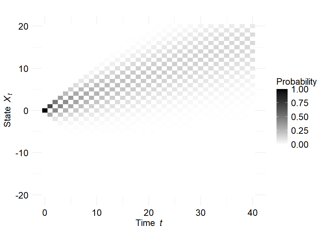
Figure 2.4: Heatmap illustrating the evolution of the probability distribution for a RW with drift.

2.2.3 Random Walk with Drift and Two Absorbing Barriers

So far, we considered RWs with unlimited evolution, that is, they never stopped. This would also imply that a response is never selected and no decision is ever made. In principle, there are two ways to determine a stop and the respective decision:

• First, one could simply stop after a predefined number of time-steps and determine the value of \({X}_t\) at that time. If it is positive, one response is selected; if it is negative, the other response is selected.
• Second, and this is the more important way for our purposes, one can stop once a particular and sufficient amount of evidence/activation has been gathered for the first time.

2.2.3.1 The Concept

The amount of sufficient evidence/activation is usually called the decision boundary and is denoted here as \(b\). As we deal with two responses, we distinguish two cases. Further sampling of evidence is stopped if \[ {X}_t \geq b \quad\text{or}\quad {X}_t \leq -b\,. \] In the first case, Response 1 is selected, and in the second case, Response 2 is selected. Technically, these boundaries are called absorbing barriers, because the process terminates once they are hit (i.e., the process is absorbed by the boundary). The time-point \(t\) where this happens the first time is called the first-passage time and it is one of the most important quantities for our purposes. The second important quantity are the frequencies with which the upper and the lower boundary \(b\) and \(-b\) are hit.

Of course we can simply simulate a large amount of RWs and determine these quantities. Figure 2.5 visualizes 10000 RWs with \(p=0.65\) and \(b=10\). There are several things to note in this figure. First, many of the RWs terminate at the upper boundary. This is, of course, to be expected when the probability of moving upward is \(p>0.5\). Second, due to the stochastic nature, some RWs also terminate at the lower boundary. With \(p>0.5\), this would implicate selection of the wrong response.⁶ Finally, for the RWs terminating at the upper and lower boundary, we have plotted bars proportional in height to the frequency of the respective first-passage time.⁷ Note that the shape of the resulting distribution looks already similar to the observed shape of RTs . If you do not know how RTs are typically distributed, do Exercise 3 in Section 1.4.3 or look at its solution (Section 1.6).

Figure 2.5: Illustration of 10000 RWs with two absorbing barriers. The bars in the upper and lower part of the panel are drawn proportionally to the frequencies of the observed first-passage times.

To explore the behavior of the RW in more detail, it is helpful to have a function that simulates a requested number of RW and determines the response choice and the respective first-passage time. The following code is one example how to do this:

simulate_RW <- function(t_max = 200,
                        n_trials = 10,
                        p_up = 0.5,
                        boundary = 10) {
  # Simulate all random walks at once:
  # Each column is one trial, each row is a time step
  steps <- matrix(
    sample(c(1, -1),
      size = t_max * n_trials,
      replace = TRUE,
      prob = c(p_up, 1 - p_up)
    ),
    nrow = t_max,
    ncol = n_trials
  )

  # Add initial 0 row for starting position at time 0
  steps <- rbind(rep(0, n_trials), steps)

  # Cumulative sum along rows (time) for each trial (column)
  X <- apply(steps, 2, cumsum)

  # Function to find first passage time and response per trial
  get_first_passage <- function(walk) {
    firstPassage <- which(walk >= boundary | walk <= -boundary)[1]
    if (is.na(firstPassage)) {
      return(c(response = NA, firstPassageTime = NA))
    } else {
      response <- sign(walk[firstPassage])
      firstPassageTime <- firstPassage - 1 # -1 because time starts at 0
      return(c(response = response, firstPassageTime = firstPassageTime))
    }
  }

  # Apply over columns (each trial)
  results <- apply(X, 2, get_first_passage)

  # Convert results to data.frame and remove NAs
  RW <- data.frame(t(results))
  RW <- na.omit(RW)

  return(RW)
}

We can now use the function simulate_RW() to generate a data frame with the requested results of RWs. To better analyze these results, we may use the following simple function to calculate the relative frequencies of RWs terminating at the upper and the lower boundary and the respective mean first-passage times:

analyze_sim <- function(data) {
  # Are there any responses at the upper boundary (1)?
  if (any(data$response == 1)) {
    # Calculate mean and frequency
    mean_resp_1 <- mean(data$firstPassageTime[data$response == 1])
    perc_resp_1 <- mean(data$response == 1)
    # Format and print
    upper <- paste0(
      "Freq. Upper responses: ", round(perc_resp_1, 2),
      "; M = ", round(mean_resp_1, 2)
    )
    print(upper)
  }

  # Are there any responses at the lower boundary (-1)?
  if (any(data$response == -1)) {
    # Calculate mean and frequency
    mean_resp_2 <- mean(data$firstPassageTime[data$response == -1])
    perc_resp_2 <- mean(data$response == -1)
    # Format and print
    lower <- paste0(
      "Freq. Lower responses: ", round(perc_resp_2, 2),
      "; M = ", round(mean_resp_2, 2)
    )
    print(lower)
  }
}

As one example, we get:

set.seed(1)
myRW <- simulate_RW(
  t_max = 100, # How many time-steps maximally?
  n_trials = 100, # How many RWs?
  p_up = 0.55, # Probability of moving up
  boundary = 10
)
head(myRW, 6) # Show first six rows

##   response firstPassageTime
## 1        1               90
## 2        1               60
## 3        1               32
## 4        1               52
## 5        1               76
## 7        1               88

analyze_sim(myRW) # Analyze RWs

## [1] "Freq. Upper responses: 0.9; M = 50.28"
## [1] "Freq. Lower responses: 0.1; M = 54.5"

2.2.3.2 Exercise: Explore the RW!

Before moving on to the next section, it is instructive to explore the behavior of RWs using the functions simulate_RW() and analyze_sim() provided above. For example, try experimenting with the probability \(p\) and the boundary \(b\). How do changes in these values affect the choice outcomes and the mean first-passage times?

Do you notice anything (perhaps unexpected) about the mean first-passage times at the upper and lower responses, which can be interpreted as correct and incorrect responses, respectively, when \(p > 0.5\)? It may also help to increase the number of trials to better observe these effects.

2.2.3.3 The Transition Matrix \(P\), Markov Chain Evolution, and First-Passage Times

We have covered so far how simulating stochastic processes using the computer is one way to study their behavior. Yet, it is also easy to see that accurate results require lots of simulations, which in turn becomes time-consuming pretty fast. However, often, but not always, there are better methods available, and the RW is a well-studied stochastic process to demonstrate this. In the following, we will introduce how we can determine quantities of interest in much faster and easier ways. These methods also provide insights into how dRiftDM works internally.

Remember that we introduced the transition matrix \(P\) of a Markov chain in the beginning of this chapter. As the RW is also a Markov chain, we can create a respective matrix for it as well (see Diederich and Busemeyer 2003; Diederich and Mallahi-Karai 2018 for more details).

For simplicity, let us assume the absorbing boundaries are at \(b=3\) and \(-b=-3\) and we stick with our example of \(P({Y}_i = 1)=p=0.6\) and \(P({Y}_i = -1)=1-p=0.4\). If the rows and columns represent the possible states that the RW \({X}_t \in \{-3,-2,-1,0,1,2,3\}\) can take, then the transition matrix is

\[ P = \begin{matrix} \scriptstyle -3 \\ \scriptstyle -2 \\ \scriptstyle -1 \\ \scriptstyle 0 \\ \scriptstyle 1 \\ \scriptstyle 2 \\ \scriptstyle 3 \end{matrix} \overset{\hspace{0.5cm} -3 \hspace{0.77cm} -2\hspace{0.77cm} -1 \hspace{0.77cm} 0 \hspace{0.92cm} 1\hspace{0.92cm} 2\hspace{0.92cm} 3 \hspace{0.7cm} }{ \begin{bmatrix} 1 & 0 & 0 & 0 & 0 & 0 & 0 \\ 0.4 & 0 & 0.6 & 0 & 0 & 0 & 0 \\ 0 & 0.4 & 0 & 0.6 & 0 & 0 & 0 \\ 0 & 0 & 0.4 & 0 & 0.6 & 0 & 0 \\ 0 & 0 & 0 & 0.4 & 0 & 0.6 & 0 \\ 0 & 0 & 0 & 0 & 0.4 & 0 & 0.6 \\ 0 & 0 & 0 & 0 & 0 & 0 & 1 \\ \end{bmatrix}}\,. \]

As in the example at the beginning of this chapter, the rows represent the current state at time \(t\), that is, where the process “comes from”, and the columns represent the state at time \(t+1\), that is, where the process will go to. For example, if the process is already absorbed, that is, it comes from -3 or +3, it will remain in this state with probability 1 (because the boundaries are absorbing). If the current state is -2 (second row), the probability of going to -3 is 0.4 and that of going to -1 is 0.6. The states “in-between” the absorbing states (e.g., -2 to 2 in our example) are called transient states. To create the matrix \(P\), we can use the following function:

# Creates a transition matrix with absorbing states b and -b,
# and the probability of moving upward p
create_transition_matrix <- function(b, p) {
  n <- 2 * b + 1 # How many states overall?
  P <- matrix(0, # Create matrix with zeros
    nrow = n,
    ncol = n
  )
  for (i in 2:(n - 1)) { # Transient states
    P[i, i - 1] <- 1 - p
    P[i, i + 1] <- p
  }
  P[1, 1] <- 1 # Absorbing states
  P[n, n] <- 1
  return(P)
}

# Create the transition matrix P
b <- 3 # Absorbing state
p <- 0.6 # P of moving up (+1)
(P <- create_transition_matrix(b, p)) # Create (and print) P

##      [,1] [,2] [,3] [,4] [,5] [,6] [,7]
## [1,]  1.0  0.0  0.0  0.0  0.0  0.0  0.0
## [2,]  0.4  0.0  0.6  0.0  0.0  0.0  0.0
## [3,]  0.0  0.4  0.0  0.6  0.0  0.0  0.0
## [4,]  0.0  0.0  0.4  0.0  0.6  0.0  0.0
## [5,]  0.0  0.0  0.0  0.4  0.0  0.6  0.0
## [6,]  0.0  0.0  0.0  0.0  0.4  0.0  0.6
## [7,]  0.0  0.0  0.0  0.0  0.0  0.0  1.0

Once \(P\) is created, we can also use it to simulate a RW from this transition matrix, just as we did for the sunny and rainy weather in the very beginning of this chapter. For simplicity, the following function that simulates a RW assumes the starting point to be in the middle of the two boundaries. Figure 2.6 visualizes one RW.

par(mar = c(4, 4, 1, 1), cex = 1.3)

# This function simulates a RW from the transition matrix P
simulate_RW_from_P <- function(P,
                               start_index = ceiling(nrow(P) / 2),
                               T_max = 50) {
  state_indices <- 1:nrow(P)
  RW <- integer(T_max + 1)
  RW[1] <- start_index

  for (t in 1:T_max) {
    current <- RW[t]
    if (P[current, current] == 1) break # absorbing state
    next_state <- sample(state_indices,
      size = 1,
      prob = P[current, ]
    )
    RW[t + 1] <- next_state
  }

  # Trim unused steps and return state indices
  RW <- RW[1:(t + 1)]
  return(RW)
}

# # Simulate one RW
set.seed(5)
RW <- simulate_RW_from_P(P)

# Convert indices back to state values -3, ..., +3
states <- c(-b:b)
RW <- states[RW]

# Plot the RW
plot(0:(length(RW) - 1),
  RW,
  type = "l",
  ylim = c(-b, b),
  xlim = c(0, 20),
  xlab = expression(plain("Time ") ~ italic(t)),
  ylab = expression(italic(X)[italic(t)]),
  main = "RW with Absorbing Boundaries"
)
abline(
  h = c(-b:b),
  col = "gray80",
  lty = 2
)
abline(
  v = c(0:50),
  col = "gray80",
  lty = 2
)
abline(h = c(-b, b))

Figure 2.6: Simulation of one RW from the transition matrix \(P\).

You might now wonder why we introduced the transition matrix \(P\) for the random walk. After all, we were already able to simulate a random walk without it, and you might even find the function simulate_RW_from_P() less elegant than simulate_RW(). However, having the matrix \(P\) at hand provides an entry to more powerful methods for analyzing RWs while sill being based on (rather simple) matrix algebra. Assume that a row vector \(X_0\) describes the state of a RW at \(t=0\) in terms of probabilities. For example, if the RW is supposed to start in the center of the two absorbing boundaries \(b=3\) and \(-b=-3\), then \[ X_0 = \begin{bmatrix}0&0&0&1&0&0&0\end{bmatrix}\,. \] In other words, the RW is with probability 1 in state 0 at \(t=0\). If we stick with our example and assume that \(p=0.6\), then we expect that the RW is in state +1 with probability 0.6, and in state -1 with probability 0.4 at \(t=1\), that is, we would expect \[ X_1 = \begin{bmatrix}0 & 0 & 0.4 & 0 & 0.6 & 0 & 0\end{bmatrix}\,. \] This is exactly what results from the matrix multiplication \(X_0\cdot P\): \[ \begin{aligned} X_1 &= X_0\cdot P \\\\ &=\begin{bmatrix}0&0&0&1&0&0&0\end{bmatrix}\cdot \left[\begin{array}{ccccccc} 1 & 0 & 0 & 0 & 0 & 0 & 0 \\ 0.4 & 0 & 0.6 & 0 & 0 & 0 & 0 \\ 0 & 0.4 & 0 & 0.6 & 0 & 0 & 0 \\ 0 & 0 & 0.4 & 0 & 0.6 & 0 & 0 \\ 0 & 0 & 0 & 0.4 & 0 & 0.6 & 0 \\ 0 & 0 & 0 & 0 & 0.4 & 0 & 0.6 \\ 0 & 0 & 0 & 0 & 0 & 0 & 1 \\ \end{array} \right]\\\\ &= \begin{bmatrix}0 & 0 & 0.4 & 0 & 0.6 & 0 & 0\end{bmatrix}\,. \end{aligned} \] This can easily be checked with R:

# We assume that P has already been created and b = 3 (as set before)
X0 <- rep(0, b * 2 + 1) # Fill all elements with 0
X0[b + 1] <- 1 # Put a 1 in the middle element
X0 # Looks good

## [1] 0 0 0 1 0 0 0

# Now we multiply X0 with P
X1 <- X0 %*% P
X1

##      [,1] [,2] [,3] [,4] [,5] [,6] [,7]
## [1,]    0    0  0.4    0  0.6    0    0

This idea generalizes to the further times \(t>1\) as well. That is, to determine the probability distribution at \(t=2\), we calculate \[ X_2 = X_1\cdot P = X_0 \cdot P\cdot P = X_0\cdot P^2\,. \] Even more generally: If a row vector \(X_0\) gives the initial distribution of a Markov chain, then the probability distribution of the chain across states at time-point \(t\) is given by the row vector \[ X_t = X_0\cdot P^t\,. \] This approach is simple but very powerful, as it allows us to develop the probability distribution forward in time from an initial distribution using basic matrix algebra. The package expm provides the operator %^% to efficiently calculate the power of a (square) matrix. If we want to determine the probability distribution at \(t=10\), we could use the following code. Be aware of the brackets: without them, R first calculates the product X0 %*% P, which is, of course, not a square matrix and cannot be taken to its \(t\)-th power.⁸

library(expm)
X10 <- X0 %*% (P %^% 10)
X10

##           [,1]       [,2] [,3]      [,4] [,5]       [,6]     [,7]
## [1,] 0.1671455 0.04299817    0 0.1289945    0 0.09674588 0.564116

The probabilities calculated so far using \(P\) are equivalent to the occupation probabilities discussed in Section 2.2.2.3. However, we can go even further and use \(P\) to derive the distribution of first-passage times.

Recall that a first-passage time distribution describes the probability of a process \(\{X_t\}\) reaching a given boundary for the first time. We have already introduced this concept in Section 2.2.3.1 and illustrated these distributions as bars in Figure 2.5. Importantly, however, the first-passage time distributions shown earlier were based on simulations, and while simulations are a flexible and intuitive method for analyzing stochastic processes, they are also time-consuming.

We will now show better ways to determine the distribution of the first-passage times using matrix algebra and the transition matrix \(P\). Conceptually, this is done as follows:

1. We start at \(t=0\) with an initial probability distribution summarized in the vector \(X_0\). While this probability is often concentrated in one single state in the center of the boundaries, other distributions are possible.
2. We determine the next state at \(t+1\) by multiplying the current state with \(P\), that is, with the just introduced matrix product \(X_{t+1} = X_t\cdot P\).
3. We then determine how much the probability to be absorbed in \(-b\) or \(b\) increases when being compared with the previous states. This is important, as the probability of a first-passage (i.e., of being absorbed) at a particular time-point must disregard the probabilities of earlier first-passages (i.e., of having been absorbed earlier already). In other words, the probability of a first-passage at a particular time-point is the incremental increase in the overall probability at the boundary.

More formally, let \(X_0\) be the initial probability distribution at \(t=0\), and \(P\) be a corresponding Markov chain transition matrix with absorbing states at \(-b\) and \(b\). At each time-step \(t>0\), the state distribution is calculated as \[ X_t = X_{t-1}\cdot P\,. \] The first-passage time distributions \(f_t^{+}\) and \(f_t^{-}\) for absorption at \(b\) and \(-b\) are defined as \[\begin{equation} \begin{aligned} f_t^+ &= P(\text{first absorption in $b$ at time-point $t$}) \\ \text{and }f_t^- &= P(\text{first absorption in $-b$ at time-point $t$})\,. \end{aligned} \end{equation}\] Setting \[ f_t^+ = X_{t;2b+1}\text{ and }f_t^- = X_{t;1}\,, \] where the second index refers to the last and first element of the vector \(Z_t\), respectively, we can then calculate the probabilities as \[\begin{equation} f_t^+ = X_{t;2b+1} - X_{t-1;2b+1}\text{ and }f_t^- = X_{t;1} - X_{t-1;1} \,. \end{equation}\]

Calculating these distributions with R is straightforward. We stick with our example of absorbing boundaries at \(b=3\) and \(-b=-3\) and the probability of moving one step up as \(p=0.6\). We have already created the transition matrix \(P\) and the initial state \(X_0\) above. We then calculate the distribution for the time-steps \(t\in \{1,\ldots,t_{max}\}\) via Markov chain evolution and extract the distributions of the first-passage times by considering the differences in the probability mass at each absorbing state between two successive steps with the R-function diff(). For comparison, we add simulation based probabilities with our earlier function simulate_RW(). Additionally, to underline the benefit of the Markov chain approach, we track the computation time for each method using tic() and toc() from the tictoc R package:

library(tictoc)

t_max <- 10 # How many time-steps do we consider?
n_states <- 2 * b + 1 # How many states do we have?
state <- X0 # The initial state
allStates <- state # The first row of a later matrix with all states

# Forward calculation of the states t = 1, ..., t_max
tic() # start timer
for (i in 1:t_max) {
  new_state <- state %*% P # Markov chain evolution
  allStates <- rbind(allStates, new_state) # Add to matrix
  state <- new_state # Prepare for next evolution step
}

# Now we extract the first-passage probabilities into a data frame
FPT <- data.frame(
  t = 1:t_max,
  FPT_lower = diff(allStates[, 1]),
  FPT_upper = diff(allStates[, n_states])
)
toc() # end timer

## 0.02 sec elapsed

# Add the first-passage probabilities based on simulations
FPT$FPT_lower_sim <- 0
FPT$FPT_upper_sim <- 0
n_trials <- 10000
tic() # start timer
sim_RW <- simulate_RW(
  t_max = t_max,
  n_trials = n_trials,
  p_up = p,
  boundary = b
)
toc() # end timer

## 0.17 sec elapsed

# Determine relative frequencies
freq_FPT <- table(sim_RW$response, sim_RW$firstPassageTime) / n_trials
timesteps_in_freq_FPT <- as.numeric(colnames(freq_FPT))

# Add the values to the data frame
FPT$FPT_lower_sim[timesteps_in_freq_FPT] <- freq_FPT["-1", ]
FPT$FPT_upper_sim[timesteps_in_freq_FPT] <- freq_FPT["1", ]

# Finally, we print the data frame and compare the results visually
round(FPT, 3)

##     t FPT_lower FPT_upper FPT_lower_sim FPT_upper_sim
## 1   1     0.000     0.000         0.000         0.000
## 2   2     0.000     0.000         0.000         0.000
## 3   3     0.064     0.216         0.059         0.217
## 4   4     0.000     0.000         0.000         0.000
## 5   5     0.046     0.156         0.050         0.159
## 6   6     0.000     0.000         0.000         0.000
## 7   7     0.033     0.112         0.033         0.114
## 8   8     0.000     0.000         0.000         0.000
## 9   9     0.024     0.081         0.026         0.077
## 10 10     0.000     0.000         0.000         0.000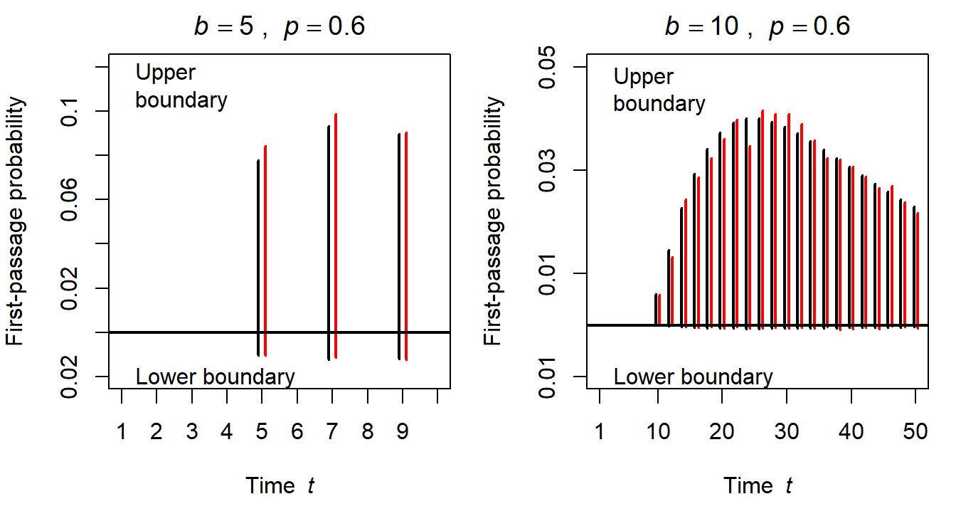

Figure 2.7 visualizes the matrix-based (black lines) and a simulation-based (red lines) distribution of first-passage times side by side. Note the discrepancies, but try yourself with larger numbers of simulated trials and explore how the simulation-based distribution approaches the matrix-based distribution, but at the expense of much more time required for the simulation.

Figure 2.7: Comparison of analytic (black lines) and simulated (red lines) distributions of first-passages. In both cases, simulations were based on 10000 trials.

How can we now calculate the proportions of upper and lower “responses” and the expected first-passage time (separately for both barriers)? The proportions are easy to calculate as they are simply the sum of the probability of first-passages for all time-steps \(t\), just separately for the lower and upper barrier:

\[ P_{+b} = \sum_t P_{+b}(t) \quad \text{and} \quad P_{-b} = \sum_t P_{-b}(t) \,. \] We can calculate these probabilities in R like this:

prob_lower <- sum(FPT$FPT_lower) # Proportion lower barrier
prob_upper <- sum(FPT$FPT_upper) # Proportion upper barrier
cat("Lower proportion: ", prob_lower, "; upper proportion: ", prob_upper)

## Lower proportion:  0.1671455 ; upper proportion:  0.564116

Does that look correct? Not really, because they do not sum to 1. We come back to this in a bit and first think about how to determine the expected (or mean) first-passage time (which we would get based on an unlimited number of simulated RWs). Basically, they are expected values, that is, we sum the products of time-values \(t\) and their probability and get \[\begin{equation} \begin{aligned} \mathbb{E}(f^+_t) & =\sum_t t\cdot P_{+b}(t) \\ \text{and }\mathbb{E}(f^-_t) & =\sum_t t\cdot P_{-b}(t)\,. \end{aligned} \end{equation}\] Doing this in R gives us:

fpt_lower <- sum(FPT$t * FPT$FPT_lower)
fpt_upper <- sum(FPT$t * FPT$FPT_upper)
cat("Lower FPT: ", fpt_lower, "; upper FPT: ", fpt_upper)

## Lower FPT:  0.869634 ; upper FPT:  2.935015

Altough it sounds straightforward, something seems wrong here as well. Why? Remember what we realized about mean first-passage times for upper and lower responses previously in this chapter. The missing point here is that we need to condition these values on whether they belong to RWs reaching the upper or the lower boundary. This means, we need to calculate \[\begin{equation} \begin{aligned} \mathbb{E}(f^+_t|+b) &= \frac{\sum_t t\cdot P_{+b}(t)}{\sum_t P_{+b}(t)} \\ \text{and }\mathbb{E}(f^-_t|-b) &= \frac{\sum_t t\cdot P_{-b}(t)}{\sum_t P_{-b}(t)}\,, \end{aligned} \end{equation}\] where the denominator is nothing else than the overall proportion of reaching the upper and lower boundary (which we have already calculated). This finally gives us:

expected_fpt_lower <- sum(FPT$t * FPT$FPT_lower) / prob_lower
expected_fpt_upper <- sum(FPT$t * FPT$FPT_upper) / prob_upper
cat("Lower FPT: ", expected_fpt_lower, "; upper FPT: ", expected_fpt_upper)

## Lower FPT:  5.202857 ; upper FPT:  5.202857

At least, the expected first-passage times are now the same for both boundaries and essentially this is how dRiftDM calculates the expected first-passage times (and their distributions). But we realized already above the sum of all response proportions is not equal to 1. Why is that? The key to this is simply that we only considered the first 10 time-steps in our example. This misses of course a number of RWs that have not been absorbed up to then and we hence missed a non-negligible portion of the “true” first-passage time distribution. This could we circumvented, however, if increase the number of time-steps we consider. We could try this again with our example from above, but now we use \(t_{max}=100\):

# Create the transition matrix P
b <- 3 # Absorbing state
p <- 0.6 # P of moving up (+1)
P <- create_transition_matrix(b, p) # Create P
t_max <- 100 # How many time-steps do we consider?
n_states <- 2 * b + 1 # How many states do we have?
X0 <- rep(0, b * 2 + 1) # Fill all elements with 0
X0[b + 1] <- 1 # Put a 1 in the middle element

state <- X0 # The initial state
allStates <- state # The first row of a later matrix with all states

# Forward calculation of the states t = 1, ..., t_max
for (i in 1:t_max) {
  new_state <- state %*% P # Markov chain evolution
  allStates <- rbind(allStates, new_state) # Add to matrix
  state <- new_state # Prepare for next evolution step
}

# Now we extract the first-passage probabilities into a data frame
FPT <- data.frame(
  t = 1:t_max,
  FPT_lower = diff(allStates[, 1]),
  FPT_upper = diff(allStates[, n_states])
)

The data frame FPT now contains the first-passage times distribution of the first 100 time-steps. We first look at the proportions of responses and see that now they almost sum up to 1, that is, we seem to have missed only very few RWs not absorbed until then:

prob_lower <- sum(FPT$FPT_lower) # Proportion lower barrier
prob_upper <- sum(FPT$FPT_upper) # Proportion upper barrier
cat("Lower proportion: ", prob_lower, "; upper proportion: ", prob_upper)

## Lower proportion:  0.2285714 ; upper proportion:  0.7714285

prob_lower + prob_upper # Almost 1 now...

## [1] 0.9999999

We then calcluate the expected first-passage times as above:

expected_fpt_lower <- sum(FPT$t * FPT$FPT_lower) / prob_lower
expected_fpt_upper <- sum(FPT$t * FPT$FPT_upper) / prob_upper
cat("Lower FPT: ", expected_fpt_lower, "; upper FPT: ", expected_fpt_upper)

## Lower FPT:  8.142847 ; upper FPT:  8.142847

They are longer now, but that is certainly as expected. Two things should be mentioned now, however:

1. These latter values are close to “optimal” estimations of the first-passage times. If you work through the following Section 2.2.3.4, you will learn a method to calculate them even easier, at least for the simple cases we are dealing with so far.
2. The maximum time \(t_{max}\) we “evaluate”, that is, how many time-steps we consider in the Markov chain evolution seems to be very important. From the examples, we can derive that \(t_{max}\) must not be too small; otherwise we simply miss “responses” and underestimate the expected first-passage times. When working with dRiftDM you will encounter a parameter t_max, which exactly determines how many time-steps are evaluated.

2.2.3.4 Excursus: Using Matrix Algebra to Determine Response Choices and Mean First-Passage-Time

We can also calculate the relative response proportion and the mean first-passage times based on \(P\) and some matrix algebra, without having to explicitly develop the Markov chain over time. For this, we slightly re-arrange \(P\) by making the last row the second row and the last column the second column. The resulting matrix is then

\[ P = \begin{matrix} \scriptstyle -3 \\ \scriptstyle 3 \\ \scriptstyle -2 \\ \scriptstyle -1 \\ \scriptstyle 0 \\ \scriptstyle 1 \\ \scriptstyle 2 \end{matrix} \overset{\hspace{0.5cm} -3 \hspace{0.92cm} 3\hspace{0.77cm} -2 \hspace{0.77cm} -1 \hspace{0.77cm} 0\hspace{0.92cm} 1\hspace{0.92cm} 2 \hspace{0.7cm} }{ \left[ \begin{array}{cc|ccccc} 1 & 0 & 0 & 0 & 0 & 0 & 0 \\ 0 & 1 & 0 & 0 & 0 & 0 & 0 \\ \hline 0.4 & 0 & 0 & 0.6 & 0 & 0 & 0 \\ 0 & 0 & 0.4 & 0 & 0.6 & 0 & 0 \\ 0 & 0 & 0 & 0.4 & 0 & 0.6 & 0 \\ 0 & 0 & 0 & 0 & 0.4 & 0 & 0.6 \\ 0 & 0.6 & 0 & 0 & 0 & 0.4 & 0 \\ \end{array} \right]}\,. \]

The re-arranged matrix can be divided into four submatrices, indicated by the vertical and horizontal line, and each submatrix has a name (the re-arranged matrix is sometimes called the canonical form of \(P\)):

\[ P = \left[ \begin{array}{c|c} P_I & 0 \\\hline R & Q \end{array} \right]\,. \] Here, \(P_I\) is a \(2\times 2\)-identity matrix, because we have two absorbing states. The zero-matrix \(0\) only contains probabilities of 0, because the process will not move anywhere, once it took an absorbing state. The \(5\times 2\)-submatrix \(R\) comprises those transient states that will end in an absorbing state in the next time-step, and the \(5\times 5\)-submatrix \(Q\) contains the probabilities of remaining within the transient states.

What the matrix \(P\), or its submatrices, do not entail is where the RW starts. For this we again define the initial state as a row vector \(X_0\). The number of entries is determined by the number of transient states, and if the process starts at state \(0\), we again have the probability \(1\) centered within the vector \[ X_0= \begin{bmatrix} 0 & 0 & 1 & 0 & 0 \end{bmatrix}\,. \]

To further determine the submatrices \(R\) and \(Q\) (which will become relevant soon), we write a small helper function to rearrange \(P\) and then take the submatrices from its result. In addition, we will already prepare the vector \(X_0\) and an identity matrix with the same dimension as \(Q\):

# Extract the submatrices from P
extract_submatrices <- function(P) {
  # Rearrange P
  P <- P[c(1, nrow(P), 2:(nrow(P) - 1)), ]
  P <- P[, c(1, ncol(P), 2:(ncol(P) - 1))]

  # Extract R and Q from the rearranged matrix P
  dimP <- nrow(P)
  R <- P[3:dimP, 1:2]
  Q <- P[3:dimP, 3:dimP]

  # pack up and pass back
  return(list(R = R, Q = Q))
}

# call the function, assign (and print) the output
submats <- extract_submatrices(P)
(R <- submats$R)

##      [,1] [,2]
## [1,]  0.4  0.0
## [2,]  0.0  0.0
## [3,]  0.0  0.0
## [4,]  0.0  0.0
## [5,]  0.0  0.6

(Q <- submats$Q)

##      [,1] [,2] [,3] [,4] [,5]
## [1,]  0.0  0.6  0.0  0.0  0.0
## [2,]  0.4  0.0  0.6  0.0  0.0
## [3,]  0.0  0.4  0.0  0.6  0.0
## [4,]  0.0  0.0  0.4  0.0  0.6
## [5,]  0.0  0.0  0.0  0.4  0.0

(X0 <- c(rep(0, times = b - 1), 1, rep(0, times = b - 1)))

## [1] 0 0 1 0 0

(I <- diag(nrow(Q)))

##      [,1] [,2] [,3] [,4] [,5]
## [1,]    1    0    0    0    0
## [2,]    0    1    0    0    0
## [3,]    0    0    1    0    0
## [4,]    0    0    0    1    0
## [5,]    0    0    0    0    1

The reason why we created these submatrices likely isn’t obvious so far. However, we can use them to simply calculate the mean first-passage time and the relative frequencies of response choices (Diederich and Busemeyer 2003; Diederich and Mallahi-Karai 2018).

Let us begin with the response choices. The \(2\times 1\)-matrix \(C\) is calculated as \[\begin{equation} C=\begin{bmatrix}P(\text{"lower"}) & P(\text{"upper"})\end{bmatrix}= X_0\cdot (I-Q)^{-1}\cdot R\,, \tag{2.6} \end{equation}\] where the first element \(C_{1,1}\) contains the relative frequency of “lower” responses and the second element \(C_{1,2}\) contains the relative frequency of “upper” responses. In this notation, \((I-Q)^{-1}\) is the inverse of the matrix \((I-Q)\) with \((I-Q)\cdot (I-Q)^{-1}=I\). The respective calculation with R is fairly easy, because the inverse of a matrix can be calculated with the function solve():

# Compute the response choices
(C <- X0 %*% solve(I - Q) %*% R)

##           [,1]      [,2]
## [1,] 0.2285714 0.7714286

The (conditional) expected values of the first-passage times can also easily be determined once \(C\) is calculate according to Equation (2.6). Specifically, let \(t\) be the random variable that describes the first-passage times, the \(2\times 1\)-matrix \(\mathbb{E}_T\) is then calculated as \[\begin{equation} \begin{aligned} \mathbb{E}_T &= \begin{bmatrix}\mathbb{E}(t|\text{"lower"}) & \mathbb{E}(t|\text{"upper"})\end{bmatrix} \\ &= [X0\cdot(I-Q)^{-2}\cdot R] \oslash C \,. \end{aligned} \tag{2.7} \end{equation}\] In this formula, \((I-Q)^{-2}\) is the matrix product \((I-Q)^{-1}\cdot (I-Q)^{-1}\), and \(\oslash\) indicates a Hadamard division, that is, the element-wise division of the matrices (rather than the standard matrix operation known from linear algebra). The respective calculation in R looks like:

(E_T <- (X0 %*% (solve(I - Q) %*% solve(I - Q)) %*% R) / C)

##          [,1]     [,2]
## [1,] 8.142857 8.142857

Note that these values are almost perfectly matching those calculated from the distribution of the first-passage times with \(t_{max}=100\) at the end of the previous section. You also see (again) the mean first-passage times for both responses are indeed the same. Figure 2.8 allows an assessment of how much the simulation-based analysis and the matrix-based analysis of the RW differ. Each data point is derived from a different amount of simulated RWs and the horizontal lines indicate the matrix-based solution. It can be seen that with 1000000 simulated RWs, the solutions are close. Yet, with less simulated RWs, remarkable differences are obvious.

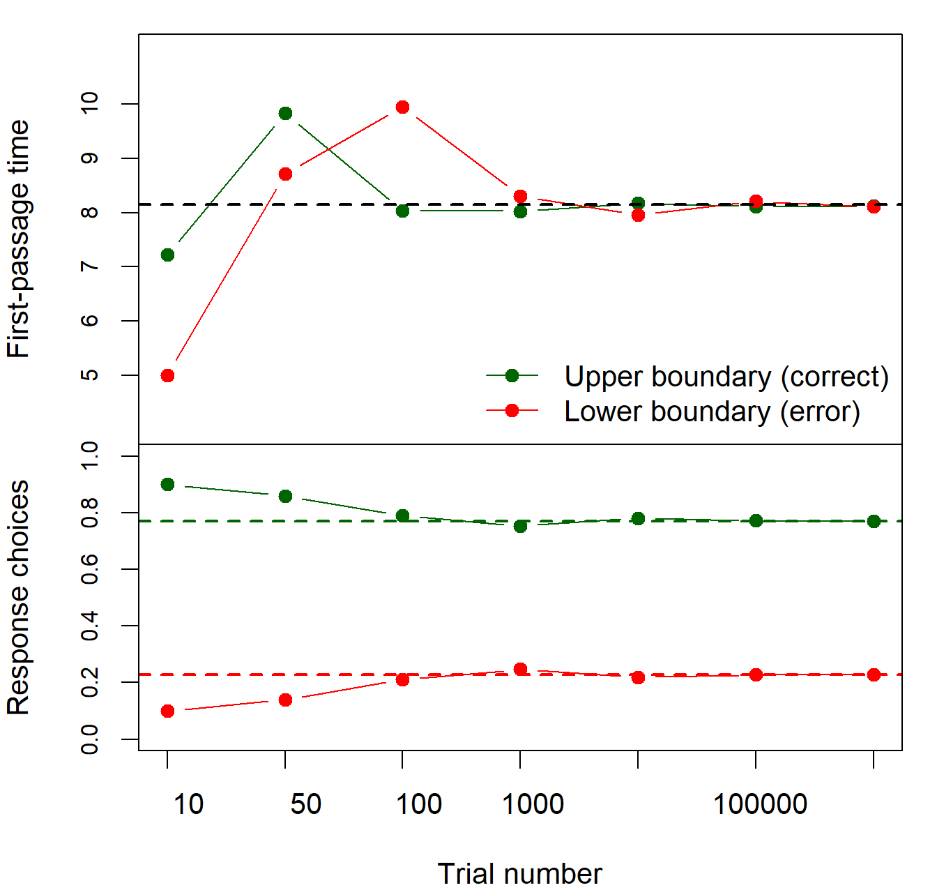
Figure 2.8: First-passage times (upper panel) and response choices (lower panel) from simulations with different numbers of trials. The black horizontal line in the upper panel indicates the analytical solution for the mean first-passage time of upper and lower boundaries, and the green and red line in the lower panel indicate the analytical solution for the response choices.

2.2.3.5 Exercise: Explore Response Choices and Mean First-Passage Times

1. Compare simulations, the method based on the distribution of first-passage times, and the matrix-based method to compute the mean first-passage times and the frequency of response choices of a RW. Play around with \(t_{max}\) (how does it affect the simulation?) and consider the differences in (computational) speed.

2. The solution presented in Equations (2.6) and (2.7) also holds when the starting point is not centered. As an exercise, try what happens to the choices and first-passage times if the starting point is centered in a different state, for example, \[ X_0=\begin{bmatrix} 0 & 0 & 0 & 1 & 0 \end{bmatrix}\,, \] or even a probability distribution of starting points is assumed, for example, \[ X_0=\begin{bmatrix} 0.1 & 0.2 & 0.4 & 0.2 & 0.1 \end{bmatrix}\,. \]

3. What is returned if you omit the \(X_0\) vector from Equations (2.6) and (2.7)? Can you interpret the result?

2.3 From Random Walks to Diffusion Models

In the previous Section 2.2, we have considered basic RWs in quite some detail. In psychological applications, one will find the DDM much more often though. There is, however, a clear relation between both models and the DDM results from a time- and state-continuous version of a RW. In other words, the RW converges to a DDM in the limit.

We will begin by relying on the symmetric RW as introduced in Section 2.2.1 to develop the stochastic component of the DDM, the Brownian motion. Then, just as we extended the symmetric RW to one with drift, we will extend the Brownian motion with a drift to describe the systematic component of a DDM. This is second core concept. The final parts concern the transition matrix \(P\) in case of a DDM, how to deal with the duration of non-decision components of processing, and extending our intuition of how dRiftDM works.

2.3.1 Wiener Process/Brownian Motion

Brownian motion describes the random motion of particles in a medium and the name goes back to the botanist Robert Brown. Its mathematical formulation was developed by Norbert Wiener, which is why Brownian motion is also known as a Wiener process in mathematics (although both terms are used interchangeably). It is a well-studied continuous-time stochastic process and can be seen as the limiting case of a symmetric RW with increasingly smaller time steps, as we will see in the next section.

More precisely, a Brownian motion \(B(t)\), \(t\geq 0\), is usually defined with the following four properties:

1. The initial condition is \(B(0)=0\).
2. For each \(0\leq s < t\), the increments \(B(t)-B(s)\) are independent of the past, that is, of \(B(u), \forall u \leq s\).
3. The distribution of \(B(t)-B(s)\) depends not on the absolute time points, but only on \(t-s\) and is \[B(t)-B(s)\sim\mathcal{N}(0,\sigma^2(t-s))\,,\] with \(\sigma^2>0\). Note that \(\sigma^2\) is just a scaling constant that determines the variance of the Brownian motion.
4. The function \(t\rightarrow B(t)\) is continuous.

From this definition it follows that \[\begin{equation} B(t)\sim \mathcal{N}(0,\sigma^2\cdot t)\,. \tag{2.8} \end{equation}\] If \(\sigma^2 = 1\), this is often called the standard Brownian motion. Note that, although being continuous, the function \(t\rightarrow B(t)\) is not differentiable: Even when you zoom in as much as you want, the trajectory stays endlessly rough and erratic (it is similar to a Weierstrass function).

While this may seem rather abstract, it can help to think of Brownian motion as the cumulative sum of normally distributed random variables. In fact, we don’t need to worry too much about the underlying mathematics of Brownian motion—as long as we have an approximation that converges to it in the limit. This is primarily because DDMs, like many other cognitive models, rely on the computer to generate model predictions, and a computer cannot handle truly time-continuous and space-continuous models. Thus, for DDMs, we always work with a discretized approximation of the stochastic process and merely ensure that our approximation meets certain properties as the discretization becomes finer and finer.

The Brownian motion is defined as above, and we will now work towards a mathematical model that fulfills this definition in the limit!

2.3.2 Approximation from a Random Walk

For RWs, the state space was always \(S = \mathbb{Z}\) and the time space was \(T=\mathbb{N}_0\). As the RW could go either up or down by exactly 1 step, the differences in steps were \(\Delta x=1\). Similarly, the time-steps were separated by \(\Delta t=1\). The general idea is now to divide this rough movement into many small steps, both in time and in space. Eventually, we consider the limiting case when \(\Delta t \rightarrow 0\) and \(\Delta x\rightarrow 0\) at the same time. However, both quantities cannot be treated independently, but must be considered in a coordinated way. With increasingly smaller and more frequent movements, the motion becomes smoother, but still random and without a clear direction. The result is the standard Brownian motion. Because Markov processes that are continuous in time and state are also called diffusion processes, this is the simplest form of a diffusion process.

We begin by subdividing the time interval we are interested in, \([0,t_{max}]\), into \(n\) smaller steps of size \(\Delta t = \frac{t_{max}}{n}\). We then modify the RW we introduced in Section 2.2.1 to make its steps at times \(t \in \{0\cdot \Delta t, 1\cdot \Delta t, 2\cdot \Delta t, \ldots, n\cdot \Delta t \}\) (with \(n\in\mathbb{N}\)). In other words, the time-steps are described as multiples of \(\Delta t\), that is, as \(k\cdot \Delta t\), \(0\leq k \leq n\). Creating the time-steps in R could look like this:

t_max <- 10 # total time (e.g., in ms)
# 1) With dt = 1 (as before)
dt <- 1.0 # time step size
(t <- seq(0, t_max, by = dt))

##  [1]  0  1  2  3  4  5  6  7  8  9 10

# 2) Smaller steps with dt = 0.5
dt <- 0.5 # time step size
(t <- seq(0, t_max, by = dt))

##  [1]  0.0  0.5  1.0  1.5  2.0  2.5  3.0  3.5  4.0  4.5  5.0  5.5  6.0  6.5  7.0
## [16]  7.5  8.0  8.5  9.0  9.5 10.0

We also modify the increments, that is, the steps for up and down movements, to be of size \(+\Delta x\) and \(-\Delta x\) (rather than \(1\) or \(-1\)). The state space \(S\) then becomes

\[S=\{\ldots,-2\cdot\Delta x, -1\cdot\Delta x, 0, + 1\cdot \Delta x,+2\cdot \Delta x,\ldots\}\,.\] This gives us, based on Equation (2.1), the (modified) stochastic difference equation

\[\begin{equation} X(t+\Delta t) = X(t) + \Delta x\cdot Y_t\text{ with }X(0)=0 \end{equation}\] to describe the evolution of the process.⁹ As before, the \(Y_i\) are independent random variables with \(P(Y_i = +1) = P(Y_i=-1) = 0.5\).

For the next steps, it is instructive to write this explicitly for some steps \(k\): \[\begin{equation} \begin{aligned} X(0) &= 0 \\ X(1\cdot\Delta t) &= X(0) + \Delta x\cdot Y_1 \\ X(2\cdot\Delta t) &= X(1\cdot \Delta t) + \Delta x\cdot Y_2 \\ &= X(0) + \Delta x\cdot Y_1 + \Delta x\cdot Y_2 \\ &= \Delta x\cdot (Y_1+Y_2)\\ X(3\cdot\Delta t) &= X(2\cdot \Delta t) + \Delta x\cdot Y_3 \\ &= X(0) + \Delta x\cdot Y_1 + \Delta x\cdot Y_2 + \Delta x\cdot Y_3\\ &= \Delta x\cdot (Y_1+Y_2+Y_3)\\ \vdots \quad&\phantom{=} \quad\quad\vdots \\ X(k\cdot\Delta t) &= X((k-1)\cdot \Delta t) + \Delta x\cdot Y_k \\ &= X(0) + \Delta x\cdot Y_1 + \Delta x\cdot Y_2 + \Delta x\cdot Y_3+\ldots+\Delta x\cdot Y_k\\ &= \Delta x\cdot (Y_1+Y_2+Y_3+\ldots+Y_k)\\ &= \Delta x\cdot \sum_{i=1}^k Y_i\,. \end{aligned} \end{equation}\] Because we write time at step \(k\) as \(t=k\cdot \Delta t \Leftrightarrow k = \frac{t}{\Delta t}\), the last instance can also be written as \[\begin{equation} \begin{aligned} X(k\cdot \Delta t) = X(t) &= \Delta x \cdot (Y_1+Y_2+Y_3+\ldots+Y_{\frac{t}{\Delta t}}) \\ &= \Delta x \cdot \sum_{i = 1}^{t /\Delta t}Y_i\,. \end{aligned} \end{equation}\] What are the expected value and the variance of \(X(t)\)? Remember from Section 2.2.1 that \(\mathbb{E}(Y_i)=0\). From this we can easily derive the expected value \[\begin{equation} \begin{aligned} \mathbb{E}[X(t)] &= \mathbb{E}\left[\Delta x \cdot \sum_{i = 1}^{t /\Delta t}Y_i\right] \\ &= \Delta x \cdot \sum_{i = 1}^{t /\Delta t}\mathbb{E}(Y_i) \\ &= 0\,. \end{aligned} \end{equation}\] The variance is calculated as \[\begin{equation} \begin{aligned} V[X(t)] &= V\left[ \Delta x \cdot \sum_{i = 1}^{t /\Delta t}Y_i \right]\\ &= (\Delta x)^2\cdot V\left[\sum_{i = 1}^{t /\Delta t}Y_i \right] \\ &= (\Delta x)^2\cdot \sum_{i = 1}^{t /\Delta t}V(Y_i) \\ &= (\Delta x)^2\cdot \frac{t}{\Delta t}\,. \end{aligned} \end{equation}\]

A useful aspect of this is that \(X(t)\) is the sum of many independent and identically distributed random variables \(Y_i\). According to the central limit theorem, the distribution of this converges to a normal distribution for \(\Delta t \rightarrow0\). This leaves us in sum with \[\begin{equation} X(t) \overset{app.}{\sim} \mathcal{N}\left(0, (\Delta x)^2\cdot \frac{t}{\Delta t}\right)\,. \tag{2.9} \end{equation}\] If we now look back at Equation (2.8), we see why this is actually useful: \(X(t)\), just like \(B(t)\), follows a normal distribution at time \(t\)!

Figure 2.9 illustrates this property and shows that with an increasing number of simulated \(Y_i\), their sum \(X(t)\) approximates a normal distribution.

Figure 2.9: Illustration that \(X(t)\) approximates a normal distribution with increasing numbers of constituent variables \(Y_i\) whose sum yield \(X(t)\). The black curve represents the theoretically expected normal distribution. For each panel, we realized \(X(t)\) 1000 times.

A still open issue that is apparent from (2.9) is that the variance of \(X(t)\) depends on the settings for \(\Delta x\) and \(\Delta t\). In fact, if we have a look at the x-axis of Figure 2.9, we see that the variance of \(X(t)\) gets larger the more \(Y_i\) constitute its sum, that is, the smaller \(\Delta t\) (\(\Delta x\) was fixed in the simulation).

This brings us to the final part. Essentially, we want \(\Delta t \rightarrow 0\) and \(\Delta x\rightarrow 0\), while keeping the variance of \(X(t)\) constant and equal to the variance of the Brownian motion as given in Equation (2.8). That is, we want \[ V[X(t)] = (\Delta x)^2\cdot\frac{t}{\Delta t}=\sigma^2\cdot t = V[B(t)]\,. \] Solving for \(\Delta x\) gives \[ \begin{aligned} & & \; (\Delta x)^2\cdot\frac{t}{\Delta t} &= \sigma^2\cdot t \\ & \Leftrightarrow & \; \frac{(\Delta x)^2}{\Delta t} &= \sigma^2 \\ & \Leftrightarrow & \; (\Delta x)^2 &= \sigma^2\cdot \Delta t \\ & \Rightarrow & \; \Delta x &= \sigma\sqrt{\Delta t} \end{aligned} \] to keep the variance \(V[X(t)]\) constant to that of the Brownian motion: \[ \begin{aligned} V[X(t)] &= (\Delta x)^2\cdot\frac{t}{\Delta t} \\ &= (\sigma\sqrt{\Delta t})^2\cdot\frac{t}{\Delta t} \\ &= \sigma^2\cdot t \\ &= V[B(t)]\,. \end{aligned} \] Figure 2.10 visualizes the trajectories of the approximated Brownian motions with different values of \(\Delta t\). Clearly, with smaller values, the trajectories become more and more smooth while still being jagged and rough.

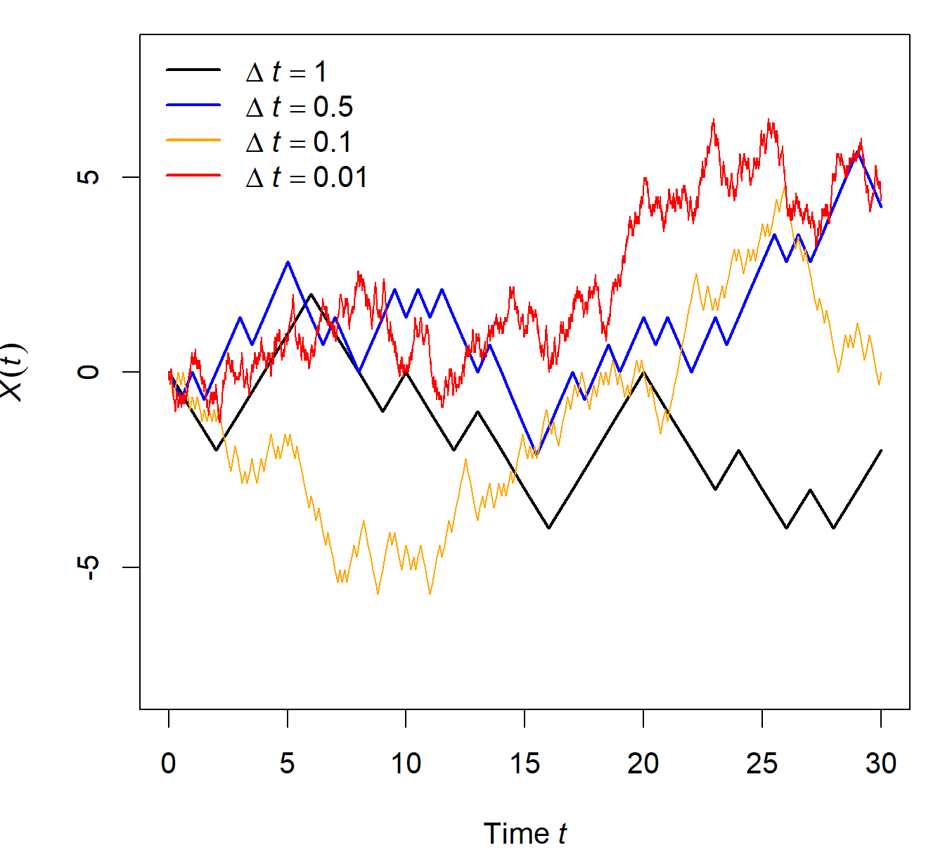
Figure 2.10: Illustration of RWs with different values for \(\Delta t\) and consequently also for \(\Delta x\). The smaller \(\Delta t\), the closer the RW approximates a Brownian motion! (\(\sigma=1\) applies for all trajectories).

Finally, let us illustrate the distribution and the variance of \(X(t)\) once more. Figure 2.11 visualizes 1000 simulated trajectories for \(\Delta t = 1\) (upper panel) and \(\Delta t = 0.1\) (lower panel; with \(\sigma=1\) in both cases). At time \(t=15\) and \(t=30\) we calculated the variance of the resulting values of \(X(t)\). The results are printed in the upper part of the panels and underlie the plotted normal distributions. Note that the values are close to the theoretically expected values of 15 and 30.

Figure 2.11: Illustration of the distribution and variance of the \(X(t)\) for two different time-step sizes \(\Delta t\). The values in the upper part of the panels are the observed variances based on 1000 simulated trajectories.

This shows that choosing the right scaling \(\Delta x=\sigma\sqrt{\Delta t}\) indeed fulfills the purpose of keeping \(V[X(t)]\) correct across the evolutions of the RW with different values of \(\Delta t\). What happens otherwise? This depends on how \(\Delta x\) is (wrongly) chosen:

• If \(\Delta x\) is chosen too large, then \(V[X(t)]\rightarrow \infty\) if \(\Delta t\rightarrow 0\), that is, the variance “explodes” to infinity (see also Figure 2.9).
• If \(\Delta x\) is chosen too small, then \(V[X(t)]\rightarrow 0\) if \(\Delta t\rightarrow 0\), that is, the variance diminishes and the process runs into a deterministic value.

In sum, we have now the knowledge on how to approximate a Brownian motion with a RW using different values of \(\Delta t\). The smaller \(\Delta t\), the more the RW converges into a Brownian motion.¹⁰ Note though, that we will never be able to match the Brownian motion exactly, because this would require an infinitesimally small value for \(\Delta t\) which our computers can’t deal with. Thus, we always work with an approximation of the Brownian motion, although those approximations are good enough and deviations from the true Brownian motion are usually too small to be relevant.

A shortcoming so far is, of course, that the process has no overall tendency to move up- or downward, as the RW is symmetric. This is also obvious from the fact that \(\mathbb{E}[X(t)]=0\). Thus, just like we have implemented the tendency for a RW to move up or down with \(p\neq 0.5\) in Section 2.2.2, the next section will treat how to implement a drift direction for the Brownian motion.

2.3.3 Brownian/Diffusion Process with Drift

The Brownian motion with drift is derived from the standard Brownian motion by superimposition with a (non-stochastic) function \(m(t)\). While \(m(t)\) can be rather arbitrary, the most typical one is a simple linear function \[m(t)=\mu\cdot t\] which is added to the Brownian motion (sometimes together with an initial starting point \(x_0\), which is for now \(x_0=0\)): \[\begin{equation} X(t)= x_0 + \mu\cdot t + \sigma B(t)\,. \end{equation}\] In this equation, \(\mu\) is termed the drift rate and \(\sigma\) is usually referred to as the diffusion constant.

This is also the basic formulation of the simple DDM as introduced by Ratcliff (1978). In fact, a Brownian motion with drift is what psychologists often call a diffusion process, and we will explore its properties in Section 3.1 in more detail.

Note that, assuming \(x_0=0\), the expected value of \(X(t)\) is now a linear function of \(t\) and hence \[ \mathbb{E}[X(t)] = \mathbb{E}[x_0 + \mu\cdot t + \sigma B(t)] = \mu\cdot t\,. \] This follows from the fact that the expected value of a Brownian motion is zero (see (2.8)). Additionally, the variance of \(X(t)\) is not altered by the drift, and is still \[ V[X(t)] = \sigma^2\cdot t\,. \] From this point of view, the drift rate can also be seen as the first derivative of the expected time-course of accumulated evidence/activation, with respect to time \(t\) (see also Cox and Miller 1965; Schwarz 2022 for this interpretation), that is, \[ \frac{d\mathbb{E}[X(t)]}{dt}=\frac{d(\mu\cdot t)}{dt}=\mu\,. \] As you can see, the drift rate \(\mu\) is independent of \(t\) and constant across time. This is why this simple model is termed time-independent. It indicates the slope of the expected time-course of accumulation and is thus the momentary rate of change. Figure 2.12 visualizes one trajectory of a diffusion process with linear drift in a way you may have encountered in articles working with DDMs.

Figure 2.12: Illustration of a diffusion process with linear drift. The dotted straight line is \(\mu\cdot t\) and the jagged gray line is a single trajectory of a Brownian motion. The jagged black line is their sum and hence a single diffusion process with linear drift.

If we want to approximate the behavior for one time-step \(\Delta t\), we can write out the increment explicitly and derive the stochastic difference equation. Thus, the discrete approximation of the continuous-time process is \[ \begin{aligned} & & X(t+\Delta t)-X(t) &= \mu\cdot \Delta t + \sigma\cdot(\underset{\Delta B(t)\sim\mathcal{N}(0, \Delta t)}{\underbrace{B(t+\Delta t) - B(t)}}) \\\\ & \Leftrightarrow & X(t+\Delta t) &= X(t) + \mu\cdot \Delta t + \sigma\cdot \Delta B(t) \\\\ & \Rightarrow & X(t+\Delta t) &= X(t) + \mu\cdot \Delta t + \sigma\cdot\sqrt{\Delta t}\cdot Z_t \end{aligned} \tag{2.10} \] with \(Z_t\sim\mathcal{N}(0,1)\) and \(X(0)=0\). Equation (2.10) is the discrete approximation of the continuous-time Brownian motion with drift and step size \(\Delta t\).¹¹ Finally, let us consider a yet different notation that highlights the continuous nature of this process. Aiming at \(\Delta t\rightarrow 0\) and borrowing from Equation (2.10), we write \[\begin{equation} \begin{aligned} \frac{X(t+\Delta t)-X(t)}{\Delta t} &= \frac{\mu\cdot \Delta t+\sigma\cdot\Delta B(t)}{\Delta t} \\\\ &= \mu + \sigma\cdot\frac{\Delta B(t)}{\Delta t}\,. \end{aligned} \end{equation}\] The term \(\frac{\Delta B(t)}{\Delta t}\) is, however, not defined as the Brownian motion is not differentiable. Rather, the stochastic differential equation is written as \[\begin{equation} dX(t) = \mu dt +\sigma dB(t)\,, \tag{2.11} \end{equation}\] Equation (2.11) roughly means that the process \(X(t)\) changes in every (infinitesimally) small time-step \(\Delta t\) by a fixed deterministic amount \(\mu dt\) and a stochastic amount \(\sigma dB(t)\) derived from a Brownian motion.¹² This equation is also the short notion of how the Brownian motion with drift can be written. Essentially then, this is (again) the simplest DDM.

To use diffusion processes as a means of modeling decisions, we again need to introduce absorbing barriers at \(b\) and \(-b\). This then yields response choices and (mean) first-passage times (or their distribution). For some simple DDMs, the probability density function of the first-passage times (i.e., their distribution) can be derived analytically. For example, if one assumes only one absorbing barrier at \(b\), the first-passage times follow a Wald (or inverse Gaussian) distribution. With two absorbing barriers, the formulas become more complicated, but are still tractable.

However, DDMs are also more general and the function \(m(t)\) does not need to be linear. For example, consider the (diminishing return) function \[ m(t) = a\cdot (1- e^{-b\cdot t})\quad\text{with }a,b>0\,. \] In this case (see Figure 2.13 for a visualization), the expected value is (again) given by \(\mathbb{E}[X(t)]=m(t)\), however, its first derivative with respect to time is now \[ \frac{d\mathbb{E}[X(t)]}{dt}=\frac{dm(t)}{dt}=a\cdot b\cdot e^{-b\cdot t}\,. \] Realize that the first derivative depends on time \(t\), but still provides the momentary rate of change for every \(t\). Thus, in this case, we have a time-dependent drift rate \(\mu(t)=a\cdot b\cdot e^{-b\cdot t}\) and the resulting DDMs are called time-dependent or non-stationary. Time-dependent DDMs will be important once we cover how to model conflict tasks, but are by far not new (e.g., Heath 1992). Critically, once we move to time-dependent DDMs, there is no analytical solution to the PDF of the first-passage times, which is why we will need to rely on numerical approximations again.

Figure 2.13: Illustration of a diffusion process with non-dependent drift. The dotted straight line is the expected time-course of evidence accumulation and the jagged gray line is a single trajectory of a Brownian motion. The jagged black is their sum and hence a single diffusion process with time-dependent drift.

2.3.4 Transition Probabilities and the Transition Matrix \(P\) for Diffusion Models

As we have elaborated in the previous sections, DDMs have an interesting relation to RWs, and the latter can be used to approximate the former. This also implies that we can again use a transition matrix \(P\) and apply the same principles as before to derive an approximation of the relative frequency of response choices and the (mean) first-passage-times for a DDM with two absorbing boundaries \(b\) and \(-b\).

The problem we have to solve to do so is: The diffusion model has the parameters \(\mu\) and \(\sigma\) (and, of course, the boundary \(b\)). The transition matrix, however, needs the transition probabilities. Hence, we must a way to express thes transition probabilities \(p\) and \(q = 1-p\) as a function of \(\mu\) and \(\sigma\) and also of \(\Delta t\) and \(\Delta x\). In fact, there are several methods to do so and we will briefly introduce two of those in the next two paragraphs.

2.3.4.1 Derivation from a Random Walk

One method to determine \(p\) and \(q\) is based on the approximation of the Brownian motion with drift from a discrete RW with increments \(\pm\Delta x\) (see Diederich and Busemeyer 2003 for details). This method relies on the scaling we have introduced above and from \(\Delta x=\sigma\cdot\sqrt{\Delta t}\) it easily follows that \(\Delta t=\frac{(\Delta x)^2}{\sigma^2}\). This implies that we cannot set \(\Delta t\) and \(\Delta x\) independent of each other, but we set \(\Delta x\) and then determine the required time-step size \(\Delta t\) from the last equation. The two transition probabilities we are interested in are then calculated as \[\begin{equation} \begin{aligned} p &= \frac{1}{2}\cdot \left(1+\frac{\mu}{\sigma}\sqrt{\Delta t}\right) \\ \text{and } q = 1-p &=\frac{1}{2}\cdot \left(1-\frac{\mu}{\sigma}\sqrt{\Delta t}\right)\,. \\ \end{aligned} \end{equation}\] If we use \(\mu = 0.2\), \(\sigma=1\), and \(\Delta x=1\) we need to set \(\Delta t=1\) and we get \(p=0.6\) and \(1=1-p=0.4\), as in the examples we used in the sections on RWs:

# Set the parameters
mu <- 0.2
sigma <- 1
dx <- 1
dt <- (dx / sigma)^2
# Then calculate p and q
p <- 0.5 * (1 + (mu / sigma) * sqrt(dt))
q <- 0.5 * (1 - (mu / sigma) * sqrt(dt))
print(paste0("p = ", p, "; q = ", q))

## [1] "p = 0.6; q = 0.4"

2.3.4.2 Discretization of the Kolmogorov Equations

A more general solution is based on the finite differences method and results from discretizing the Kolmogorov (or Fokker-Planck) Forward Equation (see Richter, Ulrich, and Janczyk 2023 for more details). The Kolmogorov Forward Equation has something in common with the forward equation introduced in Section 2.2.2.3. Basically, the Kolmogorov Forward Equations describes how the total probability mass \(P(X(t) = x)\), \(x \in S\), evolves in continuous time from an initial state at \(t=0\).¹³

In principle, this approach allows to vary all parameters (i.e., \(\Delta t\) does not necessarily depend on \(\Delta x\)), and the two transition probabilities are calculated as \[\begin{equation} \begin{aligned} p &= \frac{1}{2}\cdot \left(\frac{\sigma^2\Delta t}{(\Delta x)^2}+\frac{\mu\Delta t}{\Delta x} \right) \\ \text{and } q = 1-p &=\frac{1}{2}\cdot \left(\frac{\sigma^2\Delta t}{(\Delta x)^2}-\frac{\mu\Delta t}{\Delta x} \right)\,. \\ \end{aligned} \end{equation}\] Using the values as for the previous example, that is, \(\mu = 0.2\), \(\sigma=1\), \(\Delta x=1\), and \(\Delta t=1\) we also get \(p=0.6\) and \(q=1-p=0.4\):

# Set the parameters
mu <- 0.2
sigma <- 1
dx <- 1
dt <- (dx / sigma)^2
# Then calculate p and q
p <- 0.5 * (((sigma^2 * dt) / (dx^2)) + ((mu * dt) / (dx)))
q <- 0.5 * (((sigma^2 * dt) / (dx^2)) - ((mu * dt) / (dx)))
print(paste0("p = ", p, "; q = ", q))

## [1] "p = 0.6; q = 0.4"

Note, however, that this method also can yield unstable results and does not generally guarantee that \(0 \leq p,q \leq 1\). Just try \(\Delta x =\Delta t = 0.5\) which results in \(p=1.1\):

# Set the parameters
mu <- 0.2
sigma <- 1
dx <- 0.5
dt <- 0.5
# Then calculate p and q
p <- 0.5 * (((sigma^2 * dt) / (dx^2)) + ((mu * dt) / (dx)))
q <- 0.5 * (((sigma^2 * dt) / (dx^2)) - ((mu * dt) / (dx)))
print(paste0("p = ", p, "; q = ", q))

## [1] "p = 1.1; q = 0.9"

This can often be prevented by making sure that the step sizes are sufficiently small or by (again) setting \(\Delta t= \frac{(\Delta x)^2}{\sigma^2}\). There are also more formal conditions that guarantee stable results:

1. To ensure that \(p,q\geq 0\), the condition \(\frac{\sigma^2}{\Delta x}\geq |\mu|\) must hold, and

2. to ensure that \(p+q\leq 1\), the condition \(\Delta t\leq \frac{(\Delta x)^2}{\sigma^2}\) must hold.

2.3.4.3 Application of the Transition Matrix

Because we can specify \(p\) and \(q\) as a function of \(\mu\), \(\sigma\), \(\Delta x\), and \(\Delta t\), we can now create a transition matrix \(P\) as we did with RWs. The following function helps us create \(P\). However, unlike the previous create_transition_matrix() function in Section 2.2.3.3, we wrote the new function a bit more general, as their arguments consider \(\mu\) and \(\sigma\), and allow for a finer-grained state space (when \(\Delta x <1\)):

create_transition_matrix_for_DDM <- function(mu = 0, sigma = 1, dx = 1, b = 3) {
  # check if dx is small enough to yield reasonable p and q
  if (sigma^2 / dx < abs(mu)) {
    stop(
      "dx to large... p and q would not be between 0 and 1. ",
      "Choose a smaller value for dx."
    )
  }

  # check if we can span the range -b to b with dx
  if (b %% dx != 0) {
    stop("b divided by dx must yield an integer.")
  }

  # Calculate dt from dx to increase stability
  dt <- dx^2 / sigma^2

  # Calculate p and q (see Diederich & Busemeyer, 2003)
  p <- 0.5 * (1 + (mu / sigma) * sqrt(dt))
  q <- 0.5 * (1 - (mu / sigma) * sqrt(dt))

  # Create state space based on dx and the boundary b
  states <- seq(-b, b, by = dx)
  n <- length(states)

  # Empty matrix
  P <- matrix(0, nrow = n, ncol = n)
  colnames(P) <- rownames(P) <- format(states, nsmall = 1)

  # Setting the absorbing barriers
  P[1, 1] <- 1
  P[n, n] <- 1

  # Set the transient states
  for (i in 2:(n - 1)) {
    P[i, i - 1] <- q
    P[i, i + 1] <- p
  }
  return(P)
}

Calling this function with \(\mu = 0.2\), \(\sigma=1\), and \(\Delta x=1\) (and the implied \(\Delta t=1\)) gives us:

create_transition_matrix_for_DDM(mu = 0.2, sigma = 1, dx = 1, b = 3)

##      -3.0 -2.0 -1.0  0.0  1.0  2.0  3.0
## -3.0  1.0  0.0  0.0  0.0  0.0  0.0  0.0
## -2.0  0.4  0.0  0.6  0.0  0.0  0.0  0.0
## -1.0  0.0  0.4  0.0  0.6  0.0  0.0  0.0
##  0.0  0.0  0.0  0.4  0.0  0.6  0.0  0.0
##  1.0  0.0  0.0  0.0  0.4  0.0  0.6  0.0
##  2.0  0.0  0.0  0.0  0.0  0.4  0.0  0.6
##  3.0  0.0  0.0  0.0  0.0  0.0  0.0  1.0

Using a smaller value for the space discretization \(\Delta x\) gives us an impression of what is changed in this case:

create_transition_matrix_for_DDM(mu = 0.2, sigma = 1, dx = 0.5, b = 3)

##      -3.0 -2.5 -2.0 -1.5 -1.0 -0.5  0.0  0.5  1.0  1.5  2.0  2.5  3.0
## -3.0 1.00 0.00 0.00 0.00 0.00 0.00 0.00 0.00 0.00 0.00 0.00 0.00 0.00
## -2.5 0.45 0.00 0.55 0.00 0.00 0.00 0.00 0.00 0.00 0.00 0.00 0.00 0.00
## -2.0 0.00 0.45 0.00 0.55 0.00 0.00 0.00 0.00 0.00 0.00 0.00 0.00 0.00
## -1.5 0.00 0.00 0.45 0.00 0.55 0.00 0.00 0.00 0.00 0.00 0.00 0.00 0.00
## -1.0 0.00 0.00 0.00 0.45 0.00 0.55 0.00 0.00 0.00 0.00 0.00 0.00 0.00
## -0.5 0.00 0.00 0.00 0.00 0.45 0.00 0.55 0.00 0.00 0.00 0.00 0.00 0.00
##  0.0 0.00 0.00 0.00 0.00 0.00 0.45 0.00 0.55 0.00 0.00 0.00 0.00 0.00
##  0.5 0.00 0.00 0.00 0.00 0.00 0.00 0.45 0.00 0.55 0.00 0.00 0.00 0.00
##  1.0 0.00 0.00 0.00 0.00 0.00 0.00 0.00 0.45 0.00 0.55 0.00 0.00 0.00
##  1.5 0.00 0.00 0.00 0.00 0.00 0.00 0.00 0.00 0.45 0.00 0.55 0.00 0.00
##  2.0 0.00 0.00 0.00 0.00 0.00 0.00 0.00 0.00 0.00 0.45 0.00 0.55 0.00
##  2.5 0.00 0.00 0.00 0.00 0.00 0.00 0.00 0.00 0.00 0.00 0.45 0.00 0.55
##  3.0 0.00 0.00 0.00 0.00 0.00 0.00 0.00 0.00 0.00 0.00 0.00 0.00 1.00

We can now simply use the evolution method and the formulas introduced in Sections 2.2.3.3 and 2.2.3.4 to, for example, determine the relative response choice frequencies and the mean first-passage times.In fact, we basically use the same functions and code from these earlier sections, but need to formulate the starting condition \(X(0)\) a bit more general now. Additionally, we need to realize that all time-based measures must be multiplied with \(\Delta t\). Let us begin with a first example with \(\Delta x=\Delta t=1\):

# Set the parameters
mu <- 0.2
sigma <- 1
dx <- 1
b <- 3

# Calculate some variables needed later
dt <- dx^2 / sigma^2
states <- seq(-b, b, by = dx)
dimP <- length(states)

# Create the transition matrix P
P <- create_transition_matrix_for_DDM(mu = mu, sigma = sigma, dx = dx, b = b)

# Extract P_I, R, and Q
submatrices <- extract_submatrices(P)
R <- submatrices$R
Q <- submatrices$Q

# Create the identity matrix
I <- diag(dimP - 2)

# Create the starting distribution (centered in the middle here)
X0 <- c(rep(0, times = dimP - 2))
X0[ceiling((dimP - 2) / 2)] <- 1
X0

## [1] 0 0 1 0 0

# Calculate the relative choice frequencies and the mean first-passage times
(C <- X0 %*% solve(I - Q) %*% R)

##           -3.0       3.0
## [1,] 0.2285714 0.7714286

(E_T <- dt * (X0 %*% (solve(I - Q) %*% solve(I - Q)) %*% R) / C)

##          -3.0      3.0
## [1,] 8.142857 8.142857

In a second example, we set \(\Delta x = 0.5\) (and consequently \(\Delta t=0.25\)):

# Set the parameters
mu <- 0.2
sigma <- 1
dx <- 0.5
b <- 3

# Calculate some variables needed later
dt <- dx^2 / sigma^2
states <- seq(-b, b, by = dx)
dimP <- length(states)

# Create the transition matrix P
P <- create_transition_matrix_for_DDM(mu = mu, sigma = sigma, dx = dx, b = b)

# Extract P_I, R, and Q
submatrices <- extract_submatrices(P)
R <- submatrices$R
Q <- submatrices$Q

# Create the identity matrix
I <- diag(dimP - 2)

# Create the starting distribution (centered in the middle here)
X0 <- c(rep(0, times = dimP - 2))
X0[ceiling((dimP - 2) / 2)] <- 1
X0

##  [1] 0 0 0 0 0 1 0 0 0 0 0

# Calculate the relative choice frequencies and the mean first-passage times
(C <- X0 %*% solve(I - Q) %*% R)

##           -3.0       3.0
## [1,] 0.2307601 0.7692399

(E_T <- dt * (X0 %*% (solve(I - Q) %*% solve(I - Q)) %*% R) / C)

##          -3.0      3.0
## [1,] 8.077197 8.077197

Realize that the solutions slightly differ. However, this is expected, of course, as using smaller step sizes for \(\Delta x\) and \(\Delta t\) should yield a more accurate result.

Of course, we can also use the methods to determine the distribution of first-passage times (and calculate the response proportions and expected first-passage times from them), but we will skip this here. Instead we will next focus on how to develop a proper DDM that summarizes both decision time and non-decision time components of a response.

2.3.5 Adding the Non-Decision Time

To comply with our conceptualization visualized in Figure 1.3, we need to add the non-decision time to the first-passage time of a diffusion process (which only comprises the decision time component) to get an RT proper. According to a DDM, this non-decision time covers the duration of perceptual and motor processes that are not part of the diffusion process proper. In other words, the RT is the sum of two independent random variables, \[RT = D_{decision}+D_{t0}\,,\] where \(D_{decision}\) represents the duration of the decision, that is, the first-passage times of the underlying diffusion processes, and \(D_{t0}\) represents the duration of the non-decisional processes.

Let us assume that the first-passage times have a PDF \(f_{FPT}(t)\) representing \(D_{decision}\). In the easiest case, the non-decision time is a simple constant \(t0\).¹⁴ Then \(f_{FPT}(t)\) is just shifted (to the right), as is visualized in Figure 2.14.

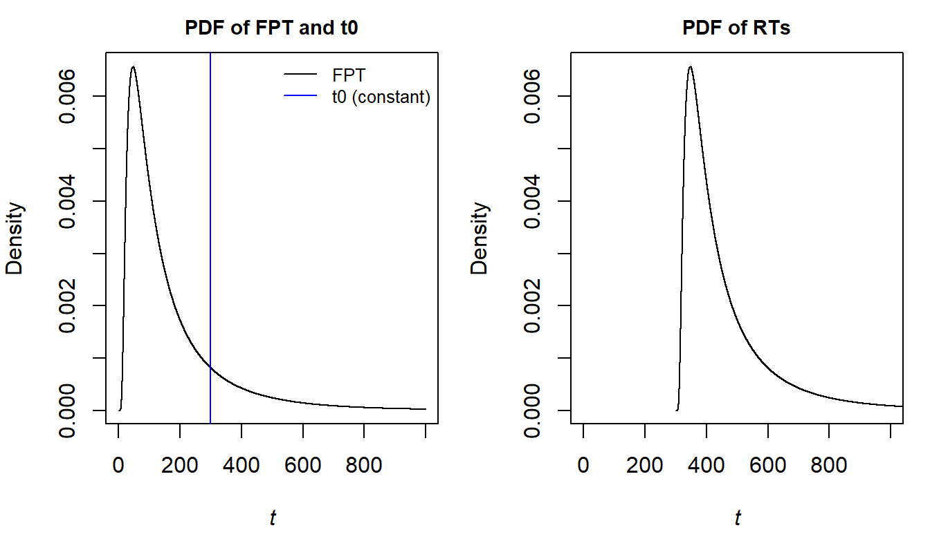
Figure 2.14: Illustration of a first-passage times PDF and a constant non-decision time \(t0\) (left panel). The constant \(t0\) leads to a shift of the first-passage times (right panel).

More realistically, the duration of the non-decision processes fluctuates as well. To account for this, the non-decision time is usually modeled as an additional random variable. Often, this random variable is assumed to follow a normal or a uniform distribution, with its PDF here denoted as \(f_{t0}(t)\). The PDF of the RT proper then results from two PDFs—from \(f_{t0}(t)\) and \(f_{FPT}(t)\). Formally, the PDF \(f_{RT}(t)\) is the convolution of \(f_{FPT}(t)\) and \(f_{t0}(t)\), \[ f_{RT}(t) = (f_{FPT}*f_{t0})(t)=\int_0^tf_{FPT}(t-\tau)\cdot f_{t0}(\tau)d\tau\,. \] Perhaps a bit more intuitive is to realize that the convolution combines two probability distributions of two (independent) random variables (here: the PDFs of the first-passage time and the non-decision time) to determine the PDF of the sum of the two random variables. For each possible total value (i.e., for each possible RT), it adds up all the ways the two random variables can yield that value as their sum. The new PDF conveys how likely each possible sum is (or more precisely: the probability that values in a particular interval are realized; the typical interpretation of a PDF). Figure 2.15 illustrates this for the case that \(t0\) follows a normal distribution. Clearly, the PDF of the RTs is shifted to the right (when compared to the PDF of the first-passage times) and it is also a bit wider and starts smoother.

Figure 2.15: Illustration of a first-passage times PDF and a normally distributed non-decision time \(t0\) (left panel) and their convolution (right panel). FPT means first-passage time.

2.3.6 What does dRiftDM do?

In the previous sections, we covered how to approximate a DDM using an RW. An important aspect of this approximation is the careful construction of the transition probabilities \(p\) and \(q\), which are then used to propagate an initial state vector \(X_0\) over time \(t\) via the transition matrix \(P\). Interestingly, this also provides some intuition about how dRiftDM works internally. In dRiftDM, a vector \(X_0\) is defined to represent the PDF of the starting condition. This PDF is then propagated forward in time \(t\) (see also Figure 2.4 for an analogy). The first-passage times of a DDM are derived by tracking the flux of probability mass at the boundaries \(b\) and \(-b\), what is similar to the method described in Section 2.2.3.3 and used to generate Figure 2.7.

There are, however, two important differences between the RW-based approach and the method implemented in dRiftDM (see also Richter, Ulrich, and Janczyk 2023). First, dRiftDM derives the transition probabilities from the Kolmogorov equations and the finite differences method. The Kolmogorov (Forward and Backward) equations (see also Cox and Miller 1965 for details) are a set of partial differential equations that result from the stochastic differential equation (see Equation (2.11)).

Second, to determine the probability distribution for each time-step \(\Delta t\), it does not simply rely on advancing the states by calculating \(X_{t + \Delta t}=X_{t}\cdot P\). This is called the explicit forward Euler scheme and it calculates the next state based on only the present state. Forward Euler is simple and makes the calculations straightforward and fast, but leads to problems and inaccuracies under several circumstances (e.g., when \(\Delta t\) is large). Instead, dRiftDM uses a scheme known as Crank-Nicolson which calculates the next state based on the mean of the old and the next state. Conceptually, this is something like \[ X_{n+1} = X_n + \frac{1}{2}\cdot \Delta t\cdot A(X_n+X_{n+1})\,, \] and in case we are interested in distributions of probabilities, \(A\) is the discrete generator matrix that contains the first and second (spatial) partial derivatives of the Kolmogorov Forward Equation. Solving the equation for \(X_{n+1}\) requires to solve a linear system for every time-step. This makes computations slower and more demanding, but the approach is more precise and stable than forward Euler. Another advantage is that this allows choosing the step sizes \(\Delta t\) and \(\Delta x\) independently of each other, and the granularity of the resulting mesh determines where the process can be evaluated at. The smaller \(\Delta t\) and \(\Delta x\), the more accurate but also time-demanding are the numerical approximations. You will encounter these settings in dRiftDM as dt and dx.

A final point of interest is that dRiftDM has no problems with time-dependent drift rates, such as already introduced in Section 2.3.3. Basically, this is achieved by letting the matrix \(P\) vary as a function of time. That is, the transition probabilities change as a function of the current drift rate \(\mu(t)\) and are dynamically adapted. In addition, also the absorbing boundaries \(b\) and \(-b\) do not necessarily have to be time-independent, that is, constant across \(t\). They can also vary as a function of time, giving \(b(t)\) and \(-b(t)\). One sometimes studied example is that the boundaries collapse with increasing time. We will briefly cover such models later in this book (see Section 5.2.2).

2.4 Summary

The information covered in this chapter should provide a fine-grained knowledge about the mathematical background of DDMs. Although it goes beyond what is essential for the application of DDMs from a practical point of view, the chapter tried to provide a good intuition on what a diffusion process actually is and how it can be numerically approximated. It also covered the concept of first-passage times which are at the heart of modeling data with a DDM in the context of psychology.

We began by introducing discrete stochastic processes and the idea of a Markov chain. For our purposes, the RW is the most basic Markov chain of interest and we analyzed its behavior in quite some detail, in particular making extensive use of the transition matrix \(P\) (see also Diederich and Busemeyer 2003 for more information). We then derived the Brownian motion, the simplest diffusion process, as a limiting case of the symmetric RW. This provided the way to the simplest DDM, with three parameters, the drift rate \(\mu\), the (absorbing) boundary \(b\), and the non-decision time \(t0\) (plus the diffusion constant \(\sigma\)). In principle, the diffusion processes of this simple DDM can also be analyzed with the transition matrix \(P\), once the transition probabilities have been derived.

In the final parts of this chapter, we provided an intuition about how dRiftDM derives the first-passage-times. Basically, the transition probabilities are derived from the Kolmogorov Forward Equation and the states are advanced to the next time-step by applying the Crank-Nicolson scheme (see Richter, Ulrich, and Janczyk 2023 for more information). There is, of course, much more to say, but this should suffice to allow understanding dRiftDM more thoroughly. We will now continue with exploring the simple DDM and its behavior by using dRiftDM.

2.5 Exercise Solutions

Explore the RW: There is no single “solution” to this exercise, but two patterns may become apparent when experimenting with the functions simulate_RW() and analyze_sim():

1. Higher boundaries lead to slower, but more accurate responses. As the boundary increases, first-passage times become longer, and the frequency of RW trajectories ending at the lower boundary decreases.

set.seed(1)
myRW1 <- simulate_RW(
  t_max = 100, # How many time-steps maximally?
  n_trials = 1000, # How many RWs?
  p_up = 0.55, # Probability of moving up
  boundary = 10
) # Boundary Value

myRW2 <- simulate_RW(
  t_max = 100, # How many time-steps maximally?
  n_trials = 1000, # How many RWs?
  p_up = 0.55, # Probability of moving up
  boundary = 15
) # Boundary Value
analyze_sim(myRW1)

## [1] "Freq. Upper responses: 0.88; M = 51.9"
## [1] "Freq. Lower responses: 0.12; M = 49.16"

analyze_sim(myRW2)

## [1] "Freq. Upper responses: 0.96; M = 64.88"
## [1] "Freq. Lower responses: 0.04; M = 58.75"

2. Higher probabilities of moving upward lead to faster and more accurate responses. As \(p\) increases, first-passage times become shorter, and the frequency of RW trajectories ending at the lower boundary decreases.

set.seed(1)
myRW1 <- simulate_RW(
  t_max = 100, # How many time-steps maximally?
  n_trials = 1000, # How many RWs?
  p_up = 0.55, # Probability of moving up
  boundary = 10
) # Boundary Value

myRW2 <- simulate_RW(
  t_max = 100, # How many time-steps maximally?
  n_trials = 1000, # How many RWs?
  p_up = 0.60, # Probability of moving up
  boundary = 10
) # Boundary Value
analyze_sim(myRW1)

## [1] "Freq. Upper responses: 0.88; M = 51.9"
## [1] "Freq. Lower responses: 0.12; M = 49.16"

analyze_sim(myRW2)

## [1] "Freq. Upper responses: 0.98; M = 43.19"
## [1] "Freq. Lower responses: 0.02; M = 32.4"

3. Mean first-passage times are identical for both boundaries, even when \(p > 0.5\)! When simulating a large number of random walks, we observe that the mean first-passage times for trajectories ending at the upper and lower boundaries are actually the same. This may seem unintuitive: if \(p > 0.5\), the walk tends to move toward the upper boundary, which might suggest that it should reach that boundary faster. However, this is not the case and this discrepancy between intuition and outcome is a great example of how cognitive models help us move beyond intuition to derive precise, testable predictions.

set.seed(1)
myRW <- simulate_RW(
  t_max = 100, # How many time-steps maximally?
  n_trials = 10000, # How many RWs?
  p_up = 0.55, # Probability of moving up
  boundary = 10
) # Boundary Value
analyze_sim(myRW)

## [1] "Freq. Upper responses: 0.88; M = 50.14"
## [1] "Freq. Lower responses: 0.12; M = 50.29"

Explore Response Choices and Mean First-Passage Times: There is no single “solution” to this exercise, but the following patterns may have become apparent.

1. The simulation approach and the approach based on the transition matrix match if we simulate a large enough amount of RWs. However, the time requirements with the transition matrix are way smaller!

b <- 5
p <- 0.55

# THE MATRIX APPROACH
tic() # requires the tictoc R package
P <- create_transition_matrix(b, p) # Create P

# get the R and Q submatrices
submats <- extract_submatrices(P)
R <- submats$R
Q <- submats$Q

# define the starting condition and an identity matrix
X0 <- c(rep(0, times = b - 1), 1, rep(0, times = b - 1))
I <- diag(nrow(Q))

# Compute the response choices and the mean first-passage times
(C <- X0 %*% solve(I - Q) %*% R)

##           [,1]      [,2]
## [1,] 0.2682826 0.7317174

(E_T <- (X0 %*% (solve(I - Q) %*% solve(I - Q)) %*% R) / C)

##          [,1]     [,2]
## [1,] 23.17174 23.17174

toc()

## 0 sec elapsed

# THE SIMULATION APPROACH
tic()
set.seed(1)
myRW <- simulate_RW(
  t_max = 100, # How many time-steps maximally?
  n_trials = 10000, # How many RWs?
  p_up = p, # Probability of moving up
  boundary = b
) # Boundary Value
analyze_sim(myRW)

## [1] "Freq. Upper responses: 0.74; M = 22.94"
## [1] "Freq. Lower responses: 0.26; M = 23.05"

toc()

## 0.47 sec elapsed

2. When the starting point is not centered, that is, when it is biased towards one of the boundaries, the frequency of RWs ending at that boundary increases. Additionally, the mean first-passage time decreases for the respective boundary.

b <- 5
p <- 0.55

P <- create_transition_matrix(b, p) # Create P
submats <- extract_submatrices(P) # get the R and Q submatrices
R <- submats$R
Q <- submats$Q

# define the biased starting condition and an identity matrix
X0 <- numeric(nrow(Q))
(X0[length(X0) * 0.35] <- 1)

## [1] 1

I <- diag(nrow(Q))

# Compute the response choices and the mean first-passage times
(C <- X0 %*% solve(I - Q) %*% R)

##           [,1]      [,2]
## [1,] 0.4774636 0.5225364

(E_T <- (X0 %*% (solve(I - Q) %*% solve(I - Q)) %*% R) / C)

##          [,1]     [,2]
## [1,] 15.52271 28.40397

3.) When defining a probability distribution of starting points which is centered around zero, the frequency of RWs ending at the lower boundary increases. Additionally, the mean first-passage times decrease, especially for the lower boundary.

b <- 5
p <- 0.55

P <- create_transition_matrix(b, p) # Create P
submats <- extract_submatrices(P) # get the R and Q submatrices
R <- submats$R
Q <- submats$Q

# define the biased starting condition and an identity matrix
idxs <- seq(0, nrow(Q) - 1, 1)
X0 <- dbinom(idxs, size = nrow(Q) - 1, prob = 0.5)
X0

## [1] 0.00390625 0.03125000 0.10937500 0.21875000 0.27343750 0.21875000 0.10937500
## [8] 0.03125000 0.00390625

I <- diag(nrow(Q))

# Compute the response choices and the mean first-passage times
# 0.268 0.731 without staring point distribution
(C <- X0 %*% solve(I - Q) %*% R)

##           [,1]      [,2]
## [1,] 0.2856585 0.7143415

# 23.17 23.17 without staring point distribution
(E_T <- (X0 %*% (solve(I - Q) %*% solve(I - Q)) %*% R) / C)

##          [,1]    [,2]
## [1,] 20.51829 21.8004

---

4. If a reminder is needed about how to calculate the expected value and the variance of a (discrete) random variable, please see here. The website is for our students in Bremen and thus in German. Of course, there are many other websites that describe the calculations in English; this one, for example. ↩︎

5. The code is also a very simple implementation to illustrate the principle. In fact, because the same values are computed multiple times, the required computation time increases exponentially. This can easily be experienced by using a too large value for \(n\). A more sophisticated programming approach uses memorization to heavily reduce computational burden.↩︎

6. Typically, DDMs are parameterized such that the expected evidence accumulation tends toward the upper boundary. In this case, the upper boundary is considered the correct response and the lower boundary the incorrect one. This is sometimes referred to as accuracy coding and is, in fact, the default in dRiftDM↩︎

7. Admittedly, we had to scale the bars at the lower boundary a bit, because otherwise they would have been too small to see them.↩︎

8. You might know that diagonalizing a matrix is in general useful to avoid extensive matrix multiplication. This means that \(P\) is expressed as \(P=U\cdot D \cdot U^{-1}\), where \(D\) is a diagonal matrix with the eigenvalues of \(P\) as entries, and \(U\) is a matrix with the columns being the eigenvectors of \(P\). The crucial point is that \(P^n=U\cdot D^n \cdot U^{-1}\) and \(D^n\) can be computed very efficiently as it simply means that the entries on the diagonal are taken to the \(n\)-th power. Using the %^% operator is nonetheless faster than implementing the diagonalized way manually in R (e.g., because expm uses a C++ backend, which is much faster than native R).↩︎

9. As we are working toward approximating a continuous-time process now, we chose to write \(X(t)\), \(X(t+\Delta t)\) and so on despite this still being a discrete case, of course. In some texts you will find \(X_t\), \(X_{t+\Delta t}\) and so on instead.↩︎

10. Note that this is an application of what is known as Donsker’s theorem.↩︎

11. You might have seen this equation in other publications on DDMs. For example, in Ulrich et al. (2015).↩︎

12. This term is not understood as a classic differential, but rather in the sense of It\(\overline{\text{o}}\)-integration. The problem is that standard (Riemann) integration is not applicable when the function is not smooth, as is the case with our stochastic processes. It\(\overline{\text{o}}\)-integration is the stochastic counterpart of the Riemann integration. It also uses a slightly different approach and comes with own rules. For example, the chain rule in standard integration is replaced by It\(\overline{\text{o}}\)’s Lemma.↩︎

13. In Section 2.2.2.3 we have introduced a forward equation to calculate the probability to end in state \(m\) when starting at state \(k\) after \(n\) steps. We already mentioned that we could treat \(m\) as a variable as well. This would give us the probability distribution of the RW when starting at \(k\) after \(n\) steps. Roughly speaking, the above forward equation is kind of the discrete version of the Kolmogorov Forward Equation.↩︎

14. Technically, this constant is also represented by a PDF. This PDF concentrates all its probability mass at a single point, so that each time a non-decision time is drawn from it, the same value results. Such a PDF is commonly known as a (shifted) Dirac delta.↩︎