4 Parameter Estimation: Basics

In Section 1.5 we gave a brief introduction into parameter estimation with simple, linear regression as the example. The idea was to find the slope $b$ and the intercept $a$ such that the model predictions best approximate the observed data.²⁴ The same applies to diffusion modeling: Parameter estimation is the process of finding values for the model parameters that yield predictions as close as possible to the observed data. This is an essential step, as good agreement between predictions and observations is one of the key criteria for evaluating the utility of a model. Additionally, once we have estimated the parameters, we can (hopefully) gain insights into the underlying cognitive processes they represent.

In the following, we will outline the basics of parameter estimation in the context of diffusion modeling. While there are many approaches to fit a model (e.g., Van Zandt 2000; Turner and Van Zandt 2012; Turner and Sederberg 2014), we will focus directly on maximum likelihood estimation, as this is the approach implemented in the dRiftDM package. Moreover, a solid understanding of maximum likelihood is a necessary foundation for more advanced techniques, such as Bayesian parameter estimation (for more information, see Held 2008; Held and Sabanés Bové 2008 and many other books).

4.1 Likelihood and Maximum Likelihood

Maximum likelihood plays a central role in statistical modeling and has a long tradition in both frequentist and Bayesian frameworks. Roughly speaking, when performing maximum likelihood estimation (MLE), we aim to find the parameter values under which the observed data are most probable.

MLE is deeply rooted in statistics and provides a set of desirable properties for the estimated parameters, often independent of the specific model. For example, if a set of regularity conditions²⁵ holds (Henze 2024), the estimates are…

consistent: Estimates become more accurate as the number of observations increases.
asymptotically normal-distributed: Their distribution approaches a normal distribution with increasing sample size.
efficient: They achieve the lowest possible variance among unbiased estimators.

In addition, likelihood theory provides a basis for evaluating model adequacy and comparing alternative models using well-established criteria such as likelihood ratio tests, AIC, and BIC. Altogether, maximum likelihood is a powerful and principled method for parameter estimation in diffusion modeling and beyond.

4.1.1 Maximum Likelihood Requires a PDF

To use MLE, we need to quantify the predictions of our model (Farrell and Lewandowsky 2018). Without model predictions, we cannot assess how plausible it is that the observed data were generated by the model. In our context, this requires the model’s predicted probability density function (PDF) of the RTs as a key ingredient. A PDF defines the probability of a continuous random variable and provides the probability that values fall into a particular range. In the context of the DDMs, the PDF specifies the probability density value of observing a particular RT and choice. For example, the PDF for the upper boundary of the Ratcliff DDM describes the probability density of a correct response occurring at a specific time. An example of such a PDF is shown in Figure 4.1.

Figure 4.1: Examplary PDF of upper boundary (i.e., correct) RTs.

From Figure 4.1, we can see that RTs associated with the upper boundary are most likely to fall between approximately 0.3 and 1.0 seconds (or 300 ms and 1,000 ms) in this example. Importantly, because we are dealing with a PDF, the values on the y-axis do not represent probabilities directly (as they would for discrete outcomes), but densities. This is because time is a continuous variable, meaning there is an infinite set of possible RTs that could, in principle, be observed. As a result, it does not make sense to assign a meaningful probability mass to a single point in time. Instead, probabilities must be computed as areas under the curve, that is, by integrating the density over an interval.²⁶

If this is unfamiliar or confusing, don’t worry. The technical details of continuous PDFs are not of too much concern here. However, it is important to understand that density values reflect relative probability, not absolute probability. In fact, this becomes apparent when we realize that density values can even exceed 1 (though they can never be negative), which would be impossible for actual probabilities. Still, we are more likely to observe RTs in areas of high density than we are to observe RTs that are associated with areas with lower density.

As discussed in Section 2.3.5, the PDF of a DDM, denoted in the following as $p_{r,k}(t)$, results from the convolution of the first passage time distribution and the non-decision time. The indices $r$ and $k$ reflect that DDMs have multiple distributions: $r$ refers to the response type (e.g., correct or incorrect; upper or lower boundary), and $k$ to a specific condition.

Importantly, for each condition $k$, the total probability across all possible responses and RTs is 1. This is formalized as:

\[ \sum_{r \in R} \left( \int_{0}^{\infty} p_{r,k}(t) \, dt \right) = 1 \quad \forall \, k \in K \]

Here, $R$ denotes the (two) possible response options (e.g., correct and incorrect), and $K$ denotes the set of conditions (e.g., congruent vs. incongruent). This essentially means that, for each condition, a response will be observed with $p=1.0$, that is with a probability of 100%.

4.1.2 From a PDF to a Likelihood

A DDM’s predicted PDFs (the part for the upper boundary was shown in Figure 4.1), provide the probability density values for a range of possible RTs and separately for the corresponding choices that could result from a single decision process. A key property of these density values is that they indicate which RTs are more “likely” (or “plausible”) than others. This already brings us close to the concept of a likelihood.

Crucially, any PDF is conditional, because it depends on the parameters of the model (and actually on the model as well). For the DDM, this means that the shape and location of the PDF are determined by parameters such as drift rate $\mu$, boundary separation $b$, and non-decision time $t0$. In the previous example, we used $\mu = 3$, $b = 0.6$, and $t0 = 0.3$ to generate the PDF. Changing any of these values would result in a different shape of the density.

Let us define $\theta$ as a vector of containing these parameter values, that is, in our example $\theta = (\mu, b, t0)$, then we can write the PDF of a DDM more formally as \[ p_{r,k}(y \mid \theta) \,, \]

where $y$ is a placeholder for observable RTs. The expression $p_{r,k}(y \mid \theta)$ still refers to a probability density, just like in the previous plots and equations. However, by writing it this way, we now make explicit that the probability density is conditional on the parameter vector $\theta$. In other words, the (conditional) PDF tells us something about how likely it is to observe a certain RT $y$ given a specific set of parameters (and a specific model).

As a prerequisite for any estimation procedure is to have obtained observed data, we will use a small set of artificial data that comes with the dRiftDM package in the following:

data <- dRiftDM::ratcliff_synth_data
head(data, n = 4)

##      RT Error Cond
## 1 0.431     0 null
## 2 0.401     0 null
## 3 0.344     0 null
## 4 0.568     0 null

For now, let us keep it simple and focus on a single data point. Figure 4.2 shows again the PDF of the Ratcliff DDM for the upper boundary, but this time also the RT of the first trial (see Figure 4.4 in Farrell and Lewandowsky 2018 for a similar plot). From the plot, we can determine the probability density value on the y-axis for the given RT. Although this value is not a probability in itself, it still provides information about the relative probability of the RT compared to all other possible RTs. As is evident, the first trial is associated with a typical RT that we could observe.

Figure 4.2: PDF created with a standard Ratcliff DDM and the RT of the first trial of the sample data set

During parameter estimation, we want to find those parameter values that enable the model to best describe the data. In the context of PDFs, this translates to the question: “Which parameter settings for $\theta$ yield the highest relative probability (i.e., PDF) given the data?” In other words, how do we need to shape the PDF of a DDM as a function of the parameters $\theta$ to yield the maximal probability density values for the data at hand? The function that helps us achieve this is called the likelihood function:

\[\mathcal{L}(\theta|y) = p(y|\theta)\]

It describes how likely it is that a certain set of data $y$ was produced by a model with the corresponding parameter set $\theta$. Importantly, the likelihood function does not introduce anything new, as it ultimately maps back to the PDF. It merely tracks how probability density values for a fixed set of data $y$ changes as a function of $\theta$.²⁷

Figure 4.3 shows the relationship between the PDF of a DDM and the likelihood function with respect to a specific parameter of the DDM, the drift rate $\mu$ (see Figure 4.6 in Farrell and Lewandowsky 2018 for a similar plot). It depicts a continuous surface, sketched out by multiple lines, with two dimensions: $t$ and $\mu$. As in the previous plots, $t$ represents the time-axis, denoting the set of potential RTs that we could observe. For a specific $\mu$, the surface yields a PDF, $p(y|\mu)$, and the PDF for $\mu = 3$ is marked in blue, representing the same PDF shown in the previous Figures 4.1 and 4.2.

The likelihood function is marked in orange and shows a line running perpendicular to the time-axis. This is the function we obtain when we assume we have a fixed set of data and wish to examine how the likelihood of the parameter $\mu$ changes in light of the data. In the present example, the line is marked at $t = 0.582$, which corresponds to the exemplary RT from above.

If we wanted to estimate the drift rate $\mu$ given the observation $t = 0.582$, we would choose that particular value of $\mu$ that leads to the highest likelihood value, that is, the parameter that yields the maximum likelihood.

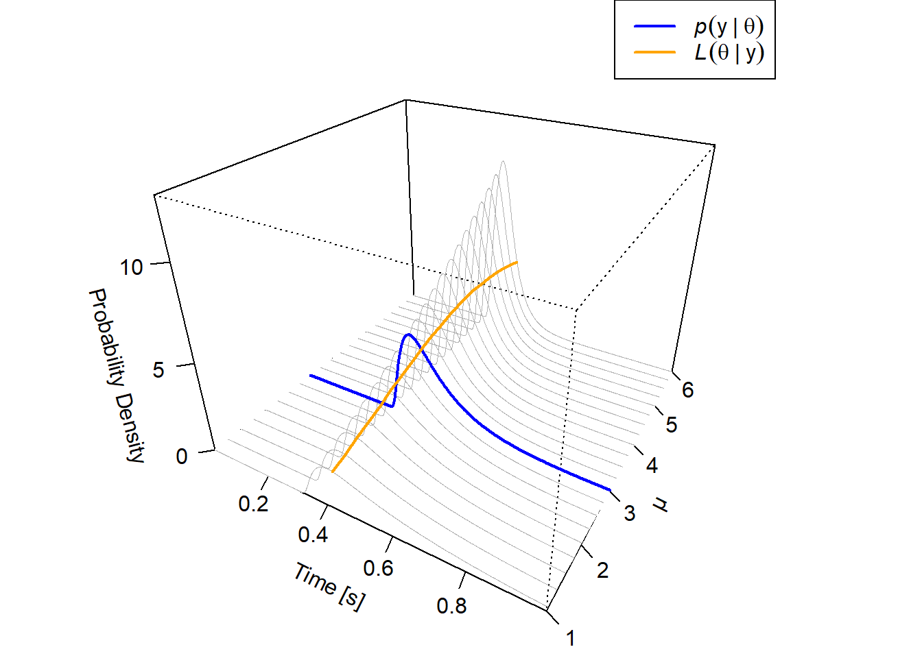
$Illustration of the relation between the PDF and the likelihood function for the drift rate $\mu$ of a DDM$

Figure 4.3: Illustration of the relation between the PDF and the likelihood function for the drift rate $\mu$ of a DDM

4.1.3 Multiple Observations and the Log-Likelihood

So far, we have explored the likelihood function using a single RT. Of course, in any data set from experimental psychology, we have multiple RTs, possibly even across multiple conditions. Fortunately, under the assumption that the individual RTs are independent given the model, we can obtain the (joint) probability density value for all the data given the parameters, which is ultimately required for the likelihood function, by multiplying the individual probability density values across all conditions and response options (Farrell and Lewandowsky 2018). That is,

\[\begin{equation} \mathcal{L}(\theta \mid y) = p(y \mid \theta) = \prod_{r \in R} \prod_{k \in K} p_{r,k}(y_{r,k})\,. \tag{4.1} \end{equation}\]

To give you an example, let’s consider the first three observations of our data set:

head(data, n = 3)

##      RT Error Cond
## 1 0.431     0 null
## 2 0.401     0 null
## 3 0.344     0 null

We can calculate the value of the likelihood function for these 3 data points by multiplying the necessary corresponding conditional probability density values: \[ \mathcal{L}(\theta \mid y) = p_{error = 0}(0.431 \mid \theta) \cdot p_{error = 0}(0.401 \mid \theta) \cdot p_{error = 0}(0.344 \mid \theta) \]

With respect to our example, we might want to calculate the likelihood value for $\mu = 3$. In this case, the necessary conditional probability density values are: \[ \begin{aligned} \mathcal{L}(\mu = 3 \mid y) &= p_{error = 0}(0.431 \mid \mu = 3) \cdot p_{error = 0}(0.401 \mid \mu = 3) \cdot p_{error = 0}(0.344 \mid \mu = 3) \\ & = 4.287 \cdot 4.818 \cdot 2.15 \approx 44.4\,. \end{aligned} \] Figure 4.4 shows how this likelihood value varies for our three data points as a function of $\mu$. The shown function is conceptually identical to the orange line in Figure 4.3, with the only difference that we now calculated the likelihood function based on multiple observations, and not based on a single observation. The likelihood value $\mathcal{L}(\mu = 3 \mid y)$ for this example is marked by black dotted lines. We will cover the R code for how to obtain the conditional probability values and thus the likelihood in Section 4.1.4.

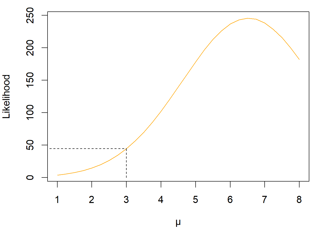
Figure 4.4: A likelihood function, created with a standard Ratcliff DDM and the first three RTs of the sample data set.

The likelihood function as written in Equation (4.1) is perfectly usable for estimating the parameters $\theta$. For example, we would estimate $\mu$ to be around 6.5 when looking at Figure 4.4. However, it involves the product of many probability density values, which can be a challenge for a computer. In fact, likelihood values are almost always very large or very small. So large or so small, that computers may struggle to represent them accurately. This problem is circumvented by considering the logarithm of the likelihood function, the log-likelihood

\[\ell(\theta \mid y) = \log\left[\mathcal{L}(\theta|y)\right] = \sum_{r \in R} \sum_{k \in K} \log\left[p_{r,k}(y_{r,k})\right]\,.\]

This has three advantages:

Taking the logarithm transforms the products implicated by the last formula into sums, which are much easier to handle computationally. Just remember a basic rule for logarithms, namely $\log(x\cdot y)=\log(x)+\log(y)$, as long as $x>0$ and $y>0$.
The logarithm of a small value results in a number with a larger absolute magnitude, for example, $\log(0.0001) = -9.21$. Conversely, taking the logarithm of a large value results in a number with smaller absolute magnitude, for example, $\log(10000) = 9.21$.
Finally, the logarithm is a monotonically increasing function, so maximizing the log-likelihood yields the same parameter estimates as maximizing the likelihood itself.

Figure 4.5 shows the logarithm of the function in Figure 4.4. That is, the log-likelihood function for our example with respect to $\mu$.

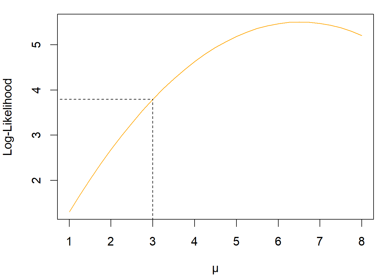
Figure 4.5: A log-likelihood function, created with a standard Ratcliff DDM and the first three RTs of the sample data set.

4.1.4 Log-Likelihood and `dRiftDM`

Using dRiftDM, we can easily compute the log-likelihood for a given set of parameters. As an example, we use the standard Ratcliff DDM here:

my_model <- ratcliff_dm(dt = 0.001, dx = 0.01)
print(my_model)

## Class(es): ratcliff_dm, drift_dm
## 
## Current Parameter Matrix:
##      muc   b non_dec
## null   3 0.6     0.3
## 
## Unique Parameters:
##      muc b non_dec
## null   1 2       3
## 
## Deriving PDFs:
##   solver: kfe
##   values: sigma=1, t_max=3, dt=0.001, dx=0.01, nt=3000, nx=200
## 
## Observed Data: NULL

In order to calculate the log-likelihood, we also need some data to condition on. For this, we will use the exemplary data set that comes with dRiftDM. Since it is already in a format compatible with dRiftDM, we can attach it directly to the model:

obs_data(my_model) <- data
print(my_model)

## Class(es): ratcliff_dm, drift_dm
## 
## Current Parameter Matrix:
##      muc   b non_dec
## null   3 0.6     0.3
## 
## Unique Parameters:
##      muc b non_dec
## null   1 2       3
## 
## Deriving PDFs:
##   solver: kfe
##   values: sigma=1, t_max=3, dt=0.001, dx=0.01, nt=3000, nx=200
## 
## Observed Data: 300 trials null

Given the data set, we can now calculate the log-likelihood for the current parameter values:

logLik(my_model)

## 'log Lik.' 189.6223 (df=3)

Calculating the Log-Likelihood by Hand: It is sometimes worth the effort to calculate something by hand to support understanding. To this end, let us calculate the log-likelihood step by step. First, we obtain the predicted PDF for the upper and lower boundaries of the classical Ratcliff DDM, given the current parameter settings. We can easily request the PDFs, along with a vector representing the time domain, using the function pdfs() of dRiftDM. Although the exact PDF values are slightly nested within a list structure, extracting and plotting them is straightforward (see Fig. 4.6).

# get the pdf values and the time domain
t_pdfs <- pdfs(my_model)
str(t_pdfs, nchar.max = 30) # shows the structure of the list

## List of 2
##  $ pdfs :List of 1
##   ..$ null:List of 2
##   .. ..$ pdf_u: num [1:3001] 1e-10 1e-10 1e-10 1e-10 1e-10 ...
##   .. ..$ pdf_l: num [1:3001] 1e-10 1e-10 1e-10 1e-10 1e-10 ...
##  $ t_vec: num [1:3001] 0 0.001 0.002 0| __truncated__ ...

# extract for easier reference
pdf_corr <- t_pdfs$pdfs$null$pdf_u # default: upper boundary == correct responses
pdf_err <- t_pdfs$pdfs$null$pdf_l # default: lower boundary == error responses
t_vec <- t_pdfs$t_vec # the time domain

# now plot both the PDF
par(mfrow = c(1, 2))
plot(pdf_corr ~ t_vec,
  type = "l",
  main = "Correct Responses",
  ylab = "Probability Density",
  xlab = "Time [s]",
  xlim = c(0, 1.5)
)
plot(pdf_err ~ t_vec,
  type = "l",
  main = "Error Responses",
  ylab = "Probability Density",
  xlab = "Time [s]",
  xlim = c(0, 1.5),
  ylim = c(0, 1)
)

Figure 4.6: PDFs of correct and incorrect responses of the classic Ratcliff DDM.

Note that the density values are much higher for correct responses than for error responses. This is because the Ratcliff DDM predicts the former to be more likely than the latter with a positive drift rate.

Next, we need to map each response in our data set to the density values. Since the density values are represented as vectors (not as continuous functions), we must convert each RT from the data set into an index so that we can access the corresponding density value by its position. To do this, we count how many steps on the time line each RT represents. In our example, we have $dt = 0.001$ seconds. Thus, an RT of $0.4$ seconds corresponds to $0.4 / 0.001 = 400$ steps on the time line, and since the time vector starts at zero, this yields the index 401.²⁸

# Get the RTs for both correct and incorrect responses
rts_corr <- data$RT[data$Error == 0]
rts_err <- data$RT[data$Error == 1]

# Turn the RTs to indices... (rounding is necessary for numerical reasons;
# If we don't do so, we might obtain indexes that are not (exactly) a digit)
idxs_corr <- round(rts_corr / 0.001) + 1
idxs_err <- round(rts_err / 0.001) + 1

# ... and access the PDF values
pdf_vals_corr <- pdf_corr[idxs_corr]
pdf_vals_err <- pdf_err[idxs_err]

Figure 4.7 visualizes the density values for 10 correct and 10 incorrect responses (showing all 300 responses would be too cluttered).

Figure 4.7: PDFs of correct and incorrect responses in the Ratcliff DDM with 10 exemplary RTs.

With the PDF values for each response at hand, we can now easily calculate the log-likelihood of the observed data set:

ll <- sum(log(c(pdf_vals_corr, pdf_vals_err)))
ll # == equal to logLik(my_model)

## [1] 189.6223

4.2 Introduction to Numerical Optimization

In the previous sections, we elaborated on what is known as the likelihood principle, which states that all information available from the data for estimating model parameters is captured by the likelihood function. This function defines a surface over the model parameters, summarizing how likely a given set of parameters $\theta$ is, given the data and model.

Once we have a way to compute the likelihood function, or its more numerically stable counterpart, the log-likelihood, the next task is to find the parameter values that maximize this function. While in some situations closed-form solutions exist and can be derived analytically, this is not the case for most models, including DDMs. Their PDFs are typically approximated numerically, and their resulting likelihood functions are complex and non-linear in the parameters. Therefore, we must rely on a computer to search for the best-fitting parameter values. This process is known as numerical optimization, in which we use iterative, numerical techniques to locate the parameter values that maximize the (log-)likelihood.

4.2.1 Visualizing the Problem

We introduced the basic principle of numerical optimization in Section 1.5, and we will now apply and extend it to MLE. Figure 4.8 illustrates an example of a log-likelihood function. It shows how the log-likelihood for the Ratcliff DDM changes when varying the drift rate $\mu$ and the decision boundary $b$, based on the same exemplary data set used in the previous section.

$Log-likelihood function of a DDM as a function of the drift rate $\mu$ and the boundary $b$.$

Figure 4.8: Log-likelihood function of a DDM as a function of the drift rate $\mu$ and the boundary $b$.

Each point on the surface shows the log-likelihood of $\theta = (\mu, b)$, quantifying how likely the respective set of parameters is given the data. The contours underneath the surface provide a 2D projection of the surface onto the base of the plot. The mode of the surface, that is, the point with the maximum log-likelihood, lies approximately at the center of the innermost contour line.

How can we now obtain those parameter values that maximize the likelihood function? One straightforward approach is to define a range for each parameter and select a set of discrete values within those ranges. We then plug each parameter combination into the model and evaluate the log-likelihood. From these values, we can easily identify the combination that yields the highest log-likelihood. This procedure is known as a grid search, as it explores the likelihood function over a grid of parameter combinations. In fact, the previous figure was created using such a grid search, evaluating 900 parameter combinations.

While grid search is simple to implement and guarantees finding the global optimum if the grid is sufficiently dense, it has two major disadvantages. First, it is computationally very expensive, especially as the number of parameters increases. For example, when having 3 parameters, we would require $30^3 = 27000$ evaluations of the log-likelihood when keeping grid density fixed. Clearly, for a model with many parameters, the number of required evaluations quickly becomes overwhelmingly high, given its exponential property. Second, it is inefficient, as we often spend time evaluating parameter regions that yield low log-likelihood values. Still, some researchers recommend grid search as an initial exploratory step. For example, the DMCfun package (Mackenzie and Dudschig 2021) performs a rough initial grid search for the peak amplitude and peak latency parameters of the automatic process of DMC (Ulrich et al. 2015), before switching to more efficient optimization algorithms.

These more efficient optimization algorithms do not evaluate the entire log-likelihood surface. In other words, they do not “see” the whole landscape, as visualized in Figure 4.8. Instead, they start at a single point and proceed in discrete steps based on specific rules, aiming to find the most optimal parameter values. You might compare these algorithms to a hiker navigating a mountain in dense fog. The goal is to reach the mountain’s peak (ideally with a rewarding view), but since the hiker is effectively blind, they rely on tapping around their immediate surroundings. Based on these discrete assessments, the hiker infers the direction in which the peak likely lies and walks in corresponding direction. During their walk, they constantly re-evaluate the curvature of the surface and adjust their movement direction accordingly.

There exist several different optimization algorithms which vary in robustness, speed, and their reliance on derivatives (of the log-likelihood function). Some common methods used in the context of (classical) DDMs include:

Gradient-based methods (e.g., Broyden–Fletcher–Goldfarb–Shanno $[$BFGS$]$ algorithm) which use information about the derivative (i.e., slope) of the likelihood function.
Derivative-free methods (e.g., Nelder-Mead simplex) which do not require the derivative (i.e., slope) of the likelihood function
Global optimization approaches (e.g., genetic algorithms) which explore the likelihood function using multiple parameter combinations.

4.2.2 Nelder-Mead and the Negative Log-Likelihood

We will begin with introducing the simplex algorithm, a classic optimization method that is relatively easy to understand and requires only the likelihood function; no derivatives of the log-likelihood function are needed.

However, before proceeding, we will convert the maximization problem into a minimization problem by considering the negative log-likelihood. By taking the negative of the log-likelihood we do not change the core problem, but simply flip it around (see Figure 4.9). In contrast to finding the parameter values that maximize the log-likelihood, we are now looking for the parameter values that minimize the negative log-likelihood.

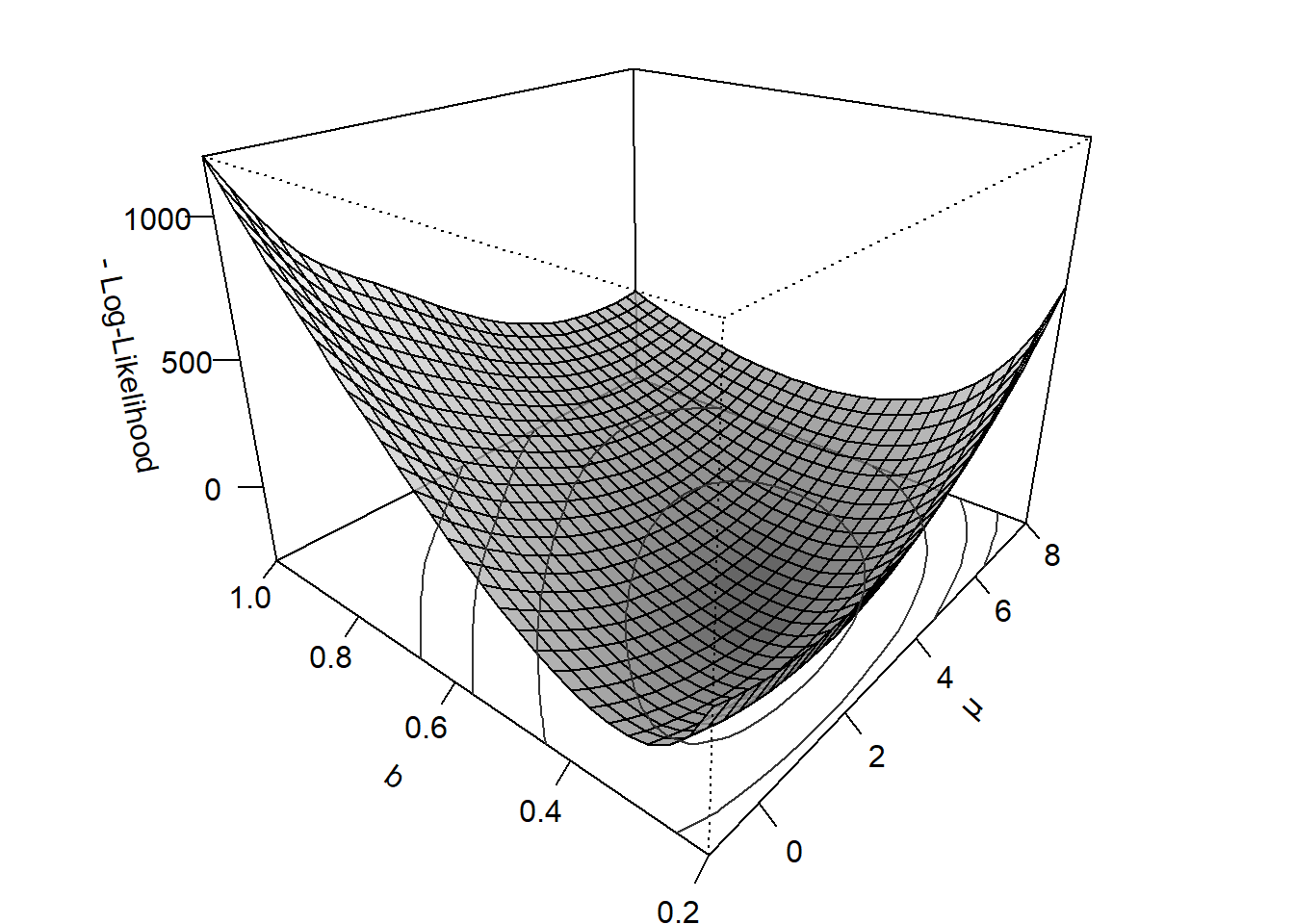
$Negative log-likelihood function of a DDM as a function of the drift rate $\nu$ and the boundary $b$.$

Figure 4.9: Negative log-likelihood function of a DDM as a function of the drift rate $\nu$ and the boundary $b$.

Why did we do that? Because many optimization algorithms are designed to minimize a function. In fact, minimization is often the default mode, and some optimization routines do not even provide an option for maximization. For this reason, you’ll often read that a model was estimated by minimizing the negative log-likelihood.²⁹

This is not a real problem, because the parameter values that maximize the log-likelihood are exactly the same as those that minimize the negative log-likelihood. Large values of the negative log-likelihood indicate a poor fit to the data, while small values indicate a better fit. Thus, the negative log-likelihood works similarly to our discrepancy function introduced in Section 1.5 and thus as a cost function.

Nelder–Mead (Nelder and Mead 1965) is a simple yet widely used optimization method. It works by moving and reshaping a simplex across the parameter space to improve the fit to the data. At each step, the algorithm attempts to improve the worst-performing point by reflecting, expanding, or contracting the simplex. A simplex is a geometric figure composed of $n+1$ points in an $n$-dimensional parameter space. If $n = 2$, a simplex is triangle. If $n = 3$, a simplex is a tetrahedron.

To illustrate, suppose we want to minimize the negative log-likelihood function for the classical Ratcliff DDM in 4.9. To this end, we provide a first guess that determines the algorithm’s starting point on the surface. In our example, this starting point is $\theta = (\mu = 1, b = 0.8)$. The goal is to move from this initial location on the curved surface toward a point in the valley, where the optimal parameters lie. Nelder–Mead places a simplex (i.e., triangle in this case) on the surface with one of the corners being our starting point . What makes a simplex useful is that it captures information about a local portion of the surface. Typically, one of its points lies higher on the surface than the other points (i.e., it yields the currently worst fit). To improve from the initial position onward, Nelder–Mead repeatedly reflects the worst point across the centroid of the remaining points, essentially flipping it to the opposite side. From this perspective, we can imagine Nelder–Mead in the present example as a triangle tumbling down the surface. Once it comes to rest in the valley, we have found the parameter values that minimize the cost function.

Figure 4.10 illustrates a Nelder–Mead run. The first three steps form the initial triangle. From there, the algorithm proceeds along a zigzagging blue path as it descends the surface. Eventually, the simplex reaches the valley floor. At this point, no further substantial improvements are possible, and the algorithm stops: the search is said to have converged.

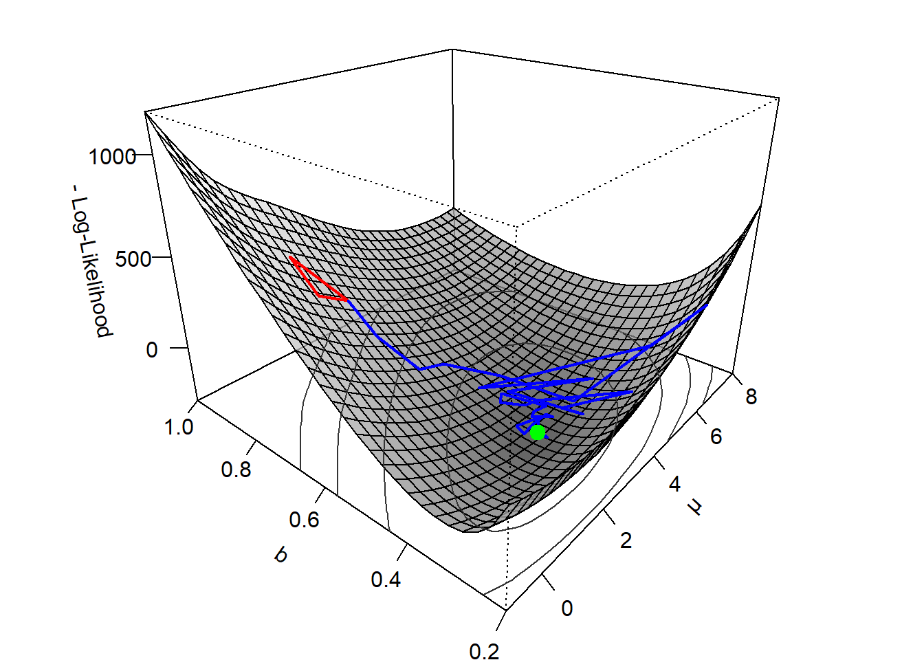
$Visualization of how a Nelder-Mead simplex algorithm determines the minimum of the negative log-likelihood function of the parameters $\nu$ and $b$ of a classic Ratcliff DDM.$

Figure 4.10: Visualization of how a Nelder-Mead simplex algorithm determines the minimum of the negative log-likelihood function of the parameters $\nu$ and $b$ of a classic Ratcliff DDM.

The Nelder–Mead procedure took 71 steps to end up in the valley in the example. In general, Nelder–Mead is relatively fast for low-dimensional problems and handles noisy functions well. However, compared to methods that use the gradient or derivative of the cost function, like BFGS, it lacks efficiency, as it necessarily has to work with an approximation of the cost function’s curvature.

4.2.3 Nelder-Mead in More Detail

While imagining Nelder–Mead as a triangle tumbling down a surface is a helpful way to grasp the basic idea of the algorithm, it is still a simplification. As introduced in the previous section, the core of the method is a simplex. Each point of the simplex represents a set of parameter values along with the corresponding value of the cost function. The algorithm then proceeds in iterations, transforming the simplex to move toward better parameter values. However, flipping the simplex is only one of several possible operations. It becomes clear that additional steps are required when we consider that the simplex must shrink to settle into a narrow region at the bottom of the valley.

Essentially, Nelder–Mead proceeds as follows:

Reflection: The worst point is reflected through the centroid of the remaining points. This “flips” the simplex, allowing the algorithm to explore the space outside the current simplex.
The function value at the reflected point is then compared to the values at the remaining points, leading to one of the following actions:
- Expansion: If the reflected point is particularly good (i.e., yields a new minimum), the algorithm tries to expand further in the same direction. If the expanded point results in an even lower minimum, it is accepted; otherwise, the original reflected point is accepted.
- Acceptance: If the reflected point is neither the best nor the worst (i.e., it yields a moderately good value), it is accepted as is.
- Contraction: If the reflected point is worse than the other (better) points, the algorithm contracts the worst point toward the centroid.
- Shrink: If none of the above steps yield improvement, the entire simplex is shrunk toward the best point.
If the function values across the simplex are sufficiently similar, the algorithm stops. Otherwise, it repeats from step 1.

These operations allow the algorithm to adaptively explore the function surface, balancing broad exploration with fine-grained local refinement.

The following code implements a version of the algorithm that prints progress information during the optimization process. We will use it in our exercise.

# x_start => numeric vector of starting values
# f => a function to minimize
# ... => additional arguments passed on to f().
# step => step size for tracing out the initial simplex
# max_iter => maximum number of iterations before giving up
# tol => tolerance, if the standard deviation of the function values across the
#        simplex falls below this value, the algorithm has converged
talking_nelder_mead <- function(x_start, f, ..., step = 0.05, max_iter = 150,
                                tol = 0.001) {
  # n are the number of parameters to optimize
  n <- length(x_start)

  # Create initial simplex: each column contains a parameter combination
  simplex <- matrix(NA, nrow = n, ncol = n + 1)
  simplex[, 1] <- x_start
  for (i in seq_len(n)) {
    x <- x_start
    x[i] <- x[i] + step
    simplex[, i + 1] <- x
  }

  # Evaluate function at each point
  values <- apply(simplex, 2, f, ...)
  cat("Initial simplex created\n")

  # run multiple iterations...
  for (iter in seq_len(max_iter)) {
    # get the index of the worst and best function evaluation
    idx_best <- which.min(values)
    idx_worst <- which.max(values)
    cat(
      "Currently, the best function evaluation is:",
      round(values[idx_best], 2), "\n"
    )

    # Centroid of best n points (excluding the worst)
    centroid <- rowMeans(simplex[, -idx_worst, drop = FALSE])

    # Reflection and function evaluation
    xr <- centroid + (centroid - simplex[, idx_worst])
    fr <- f(xr, ...)

    # now test the outcome of the reflection ...
    if (fr < values[idx_best]) {
      # if the reflection provides a new minimum, expand relative to the centroid
      cat("Expanding the reflected point\n")
      xe <- centroid + 2 * (xr - centroid) # double the distance
      fe <- f(xe, ...) # evaluate the expanded point
      # if the expanded point is even better, accept it, otherwise accept the
      # original reflection
      if (fe < fr) {
        cat("Accepting the expanded point\n")
        simplex[, idx_worst] <- xe
        values[idx_worst] <- fe
      } else {
        cat("Accepting the reflected point\n")
        simplex[, idx_worst] <- xr
        values[idx_worst] <- fr
      }
    } else if (fr < values[idx_worst]) {
      cat("Accepting the reflected point\n")
      # if the reflection provides a value in between the remaining values
      # (i.e., not worst but also not best), then accept the reflection
      simplex[, idx_worst] <- xr
      values[idx_worst] <- fr
    } else {
      # if the the reflection leads to even worse values, contract the worst
      # point towards the centroid
      cat("Contracting the worst point\n")
      xc <- centroid + 0.5 * (simplex[, idx_worst] - centroid)
      fc <- f(xc, ...)
      # test if the contraction helped...
      if (fc < values[idx_worst]) {
        cat("Accepting the contracted point\n")
        simplex[, idx_worst] <- xc
        values[idx_worst] <- fc
      } else {
        # if nothing is working, shrink everything towards the best point
        cat("Argh... Nothing works, shrinking towards the best point\n")
        xl <- simplex[, idx_best]
        idxs <- seq_len(ncol(simplex))[-idx_best]
        for (j in idxs) {
          xj <- xl + 0.5 * (simplex[, j] - xl)
          values[j] <- f(xj, ...)
          simplex[, j] <- xj
        }
      }
    }

    # Convergence check
    if (sd(values) < tol) {
      message("Converged in ", iter, " iterations.")
      break
    }
  }

  # throw a warning if the algorithm did not converge
  if (iter == max_iter && sd(values) >= tol) {
    warning("Maximum iterations reached without convergence.")
  }

  # prepare output
  idx_best <- which.min(values)
  xl <- simplex[, idx_best]
  yl <- values[idx_best]
  cat("'Best' Parameter Estimates:", round(xl, 2), "\n")
  cat("Final minimum function value:", round(yl, 2), "\n")
  list(par = xl, value = yl)
}

4.2.4 Constraining the Search Space

Nelder–Mead, in its original form, is an unconstrained optimization algorithm. This means it continues descending toward a minimum, even if that minimum corresponds to implausible or invalid parameter estimates. For example, the search might yield a negative non-decision time, which is psychologically questionable and theoretically problematic.

In practice, we often have prior intuitions about reasonable parameter values, which allows us to constrain the search space accordingly. In fact, we have already applied such a constraint implicitly in earlier figures. There, we did not plot the entire log-likelihood surface, not only because doing so is essentially impossible in higher dimensions, but also because we wanted to focus on parameter values typical for the classical Ratcliff DDM.

From a practical standpoint, constraining the optimization process improves both the efficiency of the algorithm and the reliability of parameter estimates. This is, because the likelihood surface can become flat, jagged, or undefined in extreme regions of the parameter space. By restricting the optimizer to plausible ranges, we help it avoid such problematic areas.

A common approach is to specify lower and upper bounds for each parameter. If the algorithm attempts to step outside these limits, the cost function is assigned a very large value (e.g., infinity). This effectively creates “walls” around the search space, hence the term box-constrained optimization.

An alternative is to use a penalty function: a smooth cost term that increases as parameters drift into implausible regions. This discourages the algorithm from exploring unreasonable values without imposing hard boundaries. Such soft constraints are a natural side-product in Bayesian frameworks, where priors play a similar role.

In short, constraining the search space helps ensure that the model remains interpretable and that the optimization process is stable. For this reason, many optimization functions allow for lower and upper arguments to define parameter bounds. An example is the nmkb() function in the dfoptim package, that implements a simplex algorithm with bounds.

4.2.5 Exercise: Simplex Hands-On

Now it’s your turn!

1.) Fit a DDM to real data using talking_nelder_mead().

1.1) Load the data set by Ratcliff and Rouder (1998) and select the data for one participant. Create a classical Ratcliff DDM with a variable non-decision time using dRiftDM. Fit this model to the data using your talking_nelder_mead() function. To do this, follow these steps:

Choose a discretization setting for the DDM and attach the data to the model using the functions prms_solve() and obs_data().
Write a function nll <- function(prms, model) that takes a numeric vector of parameters (prms) and a model object (model). In the body of the function, set the parameters to the model and return the negative log-likelihood.
Call talking_nelder_mead() with a set of starting values x_start and your nll() function. Make sure to pass model = <your_model> as an argument so that the optimizer can use it.
After optimization, update the parameters of your model with the best-fitting values returned by talking_nelder_mead(). Then check the model fit using calc_stats().

2.) Fit the same model using estimate_model() from dRiftDM, providing a built-in routine for Nelder–Mead optimization. Below is the general structure of the call (see the documentation and examples of estimate_model() for details):

ddm <- estimate_model(
  drift_dm_obj = ddm, # your model with data attached
  lower = c(), # lower bounds of the search space
  upper = c(), # upper bounds of the search space
  use_de_optim = FALSE, # disable DE (we will cover this later)
  use_nmkb = TRUE # use Nelder–Mead (box-constrained)
)

Run the model estimation again using estimate_model() and a fresh copy of the original DDM. Compare the resulting parameters to those from talking_nelder_mead(). Can you guess what starting values estimate_model() might use?

3.) In the exercise in Section 1.4.3, we saw that the classical DDM struggles to reproduce the delta function pattern of conflict tasks like the Simon task. We now want to check how the fit of the classical Ratcliff DDM turns out when we use it for a Simon data set. In dRiftDM we already provide a workflow for this:

simon_data <- ulrich_simon_data
model <- ratcliff_dm(t_max = 2.0, dt = 0.005, dx = 0.01, var_non_dec = TRUE)
conds(model) <- c("comp", "incomp") # more on model customization later :)
model <- modify_flex_prms(
  object = model,
  instr = "muc ~
           b ~
           non_dec ~ "
)

estimate_model_ids(
  drift_dm_obj = model,
  obs_data_ids = simon_data,
  lower = c(muc = 1, b = .3, non_dec = .1, range_non_dec = .01),
  upper = c(muc = 6, b = .9, non_dec = .5, range_non_dec = .10),
  fit_procedure_name = "simon_class_ddm", # a label to identify the fits
  fit_path = getwd(), # a location to save the individual fits
  use_de_optim = FALSE, # no DE (see the advanced optimization techniques later)
  use_nmkb = TRUE # but Nelder-Mead
)

all_fits <- load_fits_ids(fit_procedure_name = "simon_class_ddm")

plot(
  calc_stats(all_fits,
    type = c("cafs", "quantiles", "delta_funs"),
    minuends = "incomp", subtrahends = "comp"
  )
)

Try to understand the code and run it.

4.) Adapt the previous code so that it works with DMC.

4.2.6 The Troubles With Local Minima

One of the main challenges in numerical optimization is the presence of local minima, which are points in the parameter space where the objective function reaches a low value, but not the lowest possible value (i.e., not the global minimum). If the optimization algorithm gets stuck in one of these, it may converge to a suboptimal solution.

In such cases, the cost function no longer resembles a blanket sagging into a single valley. Instead, it looks more like a mountain range, with many peaks and valleys. The final result then depends heavily on the starting values and the specific behavior of the optimization algorithm. Figure 4.11 shows a negative log-likelihood surface for DMC, based on a small synthetic data set. It shows two parameters that are known to be difficult to estimate: the peak latency $\tau$ and the shape of the starting point distribution $\alpha$.

$Negative log-likelihood for DMC as a function of the parameters $\tau$ and $\alpha$.$

Figure 4.11: Negative log-likelihood for DMC as a function of the parameters $\tau$ and $\alpha$.

As is evident, the function exhibits two minima. One lies on the right edge of the plot, associated with large $\tau$ values. The other appears on the left side of the plot, marked by a sharp drop for small $\tau$ values. It is easy to see that local minima can pose a challenge for optimization algorithms, especially those like Nelder–Mead, which start from an initial point and descend toward a nearby minimum. For instance, if we provide a small value for $\tau$ as a starting point, the algorithm is likely to get “trapped” in the local minimum on the left. If instead the starting point is placed to the right of the function’s “ridge,” the algorithm may descend toward the right-hand minimum, which is lower overall.

Identifying whether an optimization algorithm has converged to a local minimum is difficult in practice, as we rarely know the global minimum in advance. However, several warning signs may indicate this problem:

The algorithm converges unusually quickly.
Another optimization run from slightly different starting points yield a different solution.
The resulting parameter estimates lead to a poor model fit.

In our experience, cost functions with multiple minima are more common than not, especially when models become more complex or the available data are limited. To mitigate the risk of local minima, several strategies can be employed:

Multiple starting points: Run the optimization algorithm several times from diverse starting values that are spread across the parameter space. If several runs converge to similar parameter values and yield a low value of the cost function, this increases our confidence that the solution is the global minimum. Alternatively, one may simply select the result with the lowest cost function value and assume it is a reasonable approximation of the best solution.
Initial grid search: Perform a coarse grid search to explore the parameter space, then initialize the optimization near the best-performing grid point. This provides a more informed starting point for local search.
Global optimization algorithms: Use more robust algorithms, such as Differential Evolution (introduced in Section 6.1.1), that are less susceptible to getting trapped in local minima. This is often the preferred approach in our own modeling work.
Bayesian inference: Switching to a Bayesian framework allows us to encode prior beliefs (ideally based on domain knowledge) about plausible parameter values. These priors can guide the search toward meaningful regions of the parameter space. We will introduce the basics of Bayesian modeling in Section 6.2.

4.2.7 Diagnostics

Now that we have covered the basics of parameter estimation, it is important to emphasize that successfully running an optimization algorithm, that is, obtaining a set of parameter values, is by no means the end of the modeling process. One should always conduct diagnostic checks and critically assess whether the obtained parameter estimates are meaningful and trustworthy. It is surprising how often articles are submitted that report only mean parameter estimates without further scrutiny. For us, basic diagnostics include (but are not limited to) the following:

Check model fit: Compare model predictions to observed data. This can include plotting observed and predicted quantiles, CAFs, or delta functions (as done in our earlier exercises). A poor fit may indicate either convergence to a local minimum or a mis-specified model.
Inspect parameter distributions: When fitting multiple participants, examining the distribution of parameter estimates can reveal issues such as boundary solutions or convergence failures. Ideally, parameter estimates should roughly follow a normal distribution. However, it is not uncommon for parameters to end up at the edges of the search space. In fact, we can see an example for this in Figure 4.11: If we would estimate $\tau$, we will likely end up with a value at upper bound of the search space, simply because the likelihood surface is lowest at the edge of the defined box.³⁰ In practical terms, this might suggest that the parameterization of the model is not working ideally, that we do not have enough data points to estimate the model parameters, or that we placed overly narrow parameter bounds.
Conduct a parameter recovery study: If parameter estimates are to be interpreted in terms of underlying psychological processes, they must be somewhat reliable. To assess this, one can simulate synthetic data using known parameter values and then re-fit the model to that synthetic data. If the estimation procedure fails to recover the original parameters, this points to problems with parameter identifiability, the estimation procedure, or both. Even a small-scale recovery study using a handful of simulated data sets can yield valuable insights. We will perform a parameter recovery for SSP in the exercise in Section 6.1.2.

Running such diagnostics is an essential part of any modeling workflow. They help ensure that the conclusions drawn from the model are not only statistically supported, but also theoretically meaningful and interpretable.

4.2.8 Treating Individual Variability

Before closing this chapter, we want to briefly discuss how to treat individual variability. In many cases, we are not dealing with data from a single individual, but from an entire group of participants. We have already encountered this during the exercises for the Simon and flanker data from Ulrich et al. (2015).

The standard procedure is to fit a model separately for each participant and then summarize results across individuals. For example, if the goal is to compare parameter estimates across experimental conditions, one can extract the individual parameter estimates and analyze them using standard statistical methods (e.g., $t$ tests or Analyses of Variance). Similarly, when evaluating model fit, it is common to average the individual model predictions. This is also the default behavior in dRiftDM when plotting summary statistics across participants. Perhaps you have already noticed the message “Aggregating across ID” in previous outputs. Of course, it is still important to inspect individual fits. While individual data can be noisy and the model fits less than perfect, checking individual fits can help determine whether group-level patterns are reflected at the individual level.

Another approach is to average the data across participants before fitting the model. While this is not compatible with standard maximum likelihood, such an approach has been used for estimation techniques based on summary statistics (e.g., Hübner and Töbel 2019; Kelber, Mittelstädt, and Ulrich 2025; Mahani et al. 2019). Aggregating the data has the advantage of reducing the computational burden, and it can yield more stable estimates when trial numbers are low (Cohen, Sanborn, and Shiffrin 2008).

However, fitting aggregated data must be approached with some caution. The parameter estimates obtained from aggregated data are not guaranteed to match the average of the individual parameter estimates. Moreover, aggregation implies that all participants can be described by the same model and that parameter estimates from the aggregated data are representative for each individual’s cognitive processes. Clearly, when individual differences are large, or when subgroups of participants qualitatively differ in their processing strategies, these assumptions may be invalid.

A third approach, hierarchical modeling, is somewhat of a mixture of the previous approaches. Rather than fitting models independently for each individual or collapsing all data into one group-level data set, hierarchical approaches assume that individual-level parameter estimates originate from group-level distributions (Shiffrin et al. 2008). This approach thus estimates parameters at both the individual and group level simultaneously. Hierarchical modeling is often implemented within a Bayesian framework, which provides the tools to specify and infer these multi-level structures more naturally. We will introduce hierarchical Bayesian parameter estimation for DDMs in Section 6.2.6.

In general, the choice of how to treat individual variability should depend on the research question and the specific DDM being used. If the goal is to test hypotheses about individual differences or perform inferential statistics across participants, fitting models at the individual level is essential. On the other hand, if the primary goal is descriptive or exploratory, fitting a model to aggregated data can be a pragmatic and informative strategy.

Regardless of the approach, it is important to be aware that each method entails both implicit and explicit assumptions. Most critically, one should never assume that a single model structure automatically fits all individuals equally well.

4.2.9 Exercise Solution

1.) Fitting a simple data set using our Nelder-Mead implementation

# Load the data and create the classical Ratcliff DDM
data <- readRDS(file.path("data", "rr98_sub.rds"))
data <- data[data$ID == 1, ]

ddm <- ratcliff_dm(dt = 0.01, dx = 0.01)
obs_data(ddm) <- data

# provide the cost function
nll <- function(prms, model) {
  coef(model) <- prms
  return(-logLik(model))
}

# does it work?
nll(
  prms = c(2, 0.5, 0.2), # muc, b, non_dec
  model = ddm
)

## 'log Lik.' 6433.443 (df=3)

# now call the Nelder-Mead implementation
result <- talking_nelder_mead(f = nll, x_start = c(2, 0.5, 0.2), model = ddm)

## Initial simplex created
## Currently, the best function evaluation is: 5763.46 
## Accepting the reflected point
## Currently, the best function evaluation is: 5763.46 
## Contracting the worst point
## Accepting the contracted point
## Currently, the best function evaluation is: 5763.46 
## Accepting the reflected point
## Currently, the best function evaluation is: 5763.46 
## Accepting the reflected point
## Currently, the best function evaluation is: 5763.46 
## Expanding the reflected point
## Accepting the reflected point
## Currently, the best function evaluation is: 5404.14 
## Accepting the reflected point
## Currently, the best function evaluation is: 5404.14 
## Accepting the reflected point
## Currently, the best function evaluation is: 5404.14 
## Contracting the worst point
## Accepting the contracted point
## Currently, the best function evaluation is: 5404.14 
## Expanding the reflected point
## Accepting the reflected point
## Currently, the best function evaluation is: 5331.3 
## Expanding the reflected point
## Accepting the expanded point
## Currently, the best function evaluation is: 5210.34 
## Expanding the reflected point
## Accepting the expanded point
## Currently, the best function evaluation is: 5133.43 
## Expanding the reflected point
## Accepting the reflected point
## Currently, the best function evaluation is: 5121.49 
## Expanding the reflected point
## Accepting the expanded point
## Currently, the best function evaluation is: 4709.39 
## Accepting the reflected point
## Currently, the best function evaluation is: 4709.39 
## Contracting the worst point
## Accepting the contracted point
## Currently, the best function evaluation is: 4709.39 
## Accepting the reflected point
## Currently, the best function evaluation is: 4709.39 
## Expanding the reflected point
## Accepting the expanded point
## Currently, the best function evaluation is: 4490.05 
## Accepting the reflected point
## Currently, the best function evaluation is: 4490.05 
## Expanding the reflected point
## Accepting the expanded point
## Currently, the best function evaluation is: 4021.66 
## Accepting the reflected point
## Currently, the best function evaluation is: 4021.66 
## Accepting the reflected point
## Currently, the best function evaluation is: 4021.66 
## Accepting the reflected point
## Currently, the best function evaluation is: 4021.66 
## Contracting the worst point
## Accepting the contracted point
## Currently, the best function evaluation is: 4021.66 
## Expanding the reflected point
## Accepting the expanded point
## Currently, the best function evaluation is: 3811.3 
## Expanding the reflected point
## Accepting the expanded point
## Currently, the best function evaluation is: 3620.13 
## Accepting the reflected point
## Currently, the best function evaluation is: 3620.13 
## Accepting the reflected point
## Currently, the best function evaluation is: 3620.13 
## Expanding the reflected point
## Accepting the reflected point
## Currently, the best function evaluation is: 3566.03 
## Accepting the reflected point
## Currently, the best function evaluation is: 3566.03 
## Contracting the worst point
## Accepting the contracted point
## Currently, the best function evaluation is: 3467.09 
## Contracting the worst point
## Accepting the contracted point
## Currently, the best function evaluation is: 3460.22 
## Expanding the reflected point
## Accepting the reflected point
## Currently, the best function evaluation is: 3439.4 
## Contracting the worst point
## Accepting the contracted point
## Currently, the best function evaluation is: 3428.11 
## Contracting the worst point
## Accepting the contracted point
## Currently, the best function evaluation is: 3409.67 
## Accepting the reflected point
## Currently, the best function evaluation is: 3409.67 
## Contracting the worst point
## Accepting the contracted point
## Currently, the best function evaluation is: 3381.37 
## Contracting the worst point
## Accepting the contracted point
## Currently, the best function evaluation is: 3381.37 
## Accepting the reflected point
## Currently, the best function evaluation is: 3381.37 
## Contracting the worst point
## Accepting the contracted point
## Currently, the best function evaluation is: 3380.78 
## Contracting the worst point
## Accepting the contracted point
## Currently, the best function evaluation is: 3377.02 
## Contracting the worst point
## Argh... Nothing works, shrinking towards the best point
## Currently, the best function evaluation is: 3375.88 
## Accepting the reflected point
## Currently, the best function evaluation is: 3375.88 
## Contracting the worst point
## Accepting the contracted point
## Currently, the best function evaluation is: 3375.88 
## Expanding the reflected point
## Accepting the reflected point
## Currently, the best function evaluation is: 3368.67 
## Accepting the reflected point
## Currently, the best function evaluation is: 3368.67 
## Accepting the reflected point
## Currently, the best function evaluation is: 3368.67 
## Contracting the worst point
## Accepting the contracted point
## Currently, the best function evaluation is: 3368.67 
## Contracting the worst point
## Accepting the contracted point
## Currently, the best function evaluation is: 3368.67 
## Expanding the reflected point
## Accepting the reflected point
## Currently, the best function evaluation is: 3367.79 
## Expanding the reflected point
## Accepting the reflected point
## Currently, the best function evaluation is: 3367.77 
## Contracting the worst point
## Accepting the contracted point
## Currently, the best function evaluation is: 3367.77 
## Contracting the worst point
## Accepting the contracted point
## Currently, the best function evaluation is: 3367.77 
## Expanding the reflected point
## Accepting the expanded point
## Currently, the best function evaluation is: 3367.24 
## Expanding the reflected point
## Accepting the expanded point
## Currently, the best function evaluation is: 3365.29 
## Expanding the reflected point
## Accepting the expanded point
## Currently, the best function evaluation is: 3363.83 
## Accepting the reflected point
## Currently, the best function evaluation is: 3363.83 
## Expanding the reflected point
## Accepting the expanded point
## Currently, the best function evaluation is: 3360.3 
## Accepting the reflected point
## Currently, the best function evaluation is: 3360.3 
## Expanding the reflected point
## Accepting the reflected point
## Currently, the best function evaluation is: 3360.11 
## Expanding the reflected point
## Accepting the expanded point
## Currently, the best function evaluation is: 3357.99 
## Expanding the reflected point
## Accepting the reflected point
## Currently, the best function evaluation is: 3357.79 
## Accepting the reflected point
## Currently, the best function evaluation is: 3357.79 
## Contracting the worst point
## Accepting the contracted point
## Currently, the best function evaluation is: 3357.79 
## Contracting the worst point
## Accepting the contracted point
## Currently, the best function evaluation is: 3357.79 
## Accepting the reflected point
## Currently, the best function evaluation is: 3357.79 
## Accepting the reflected point
## Currently, the best function evaluation is: 3357.79 
## Contracting the worst point
## Accepting the contracted point
## Currently, the best function evaluation is: 3357.79 
## Contracting the worst point
## Accepting the contracted point
## Currently, the best function evaluation is: 3357.68 
## Contracting the worst point
## Accepting the contracted point
## Currently, the best function evaluation is: 3357.68 
## Expanding the reflected point
## Accepting the reflected point
## Currently, the best function evaluation is: 3357.68 
## Contracting the worst point
## Accepting the contracted point
## Currently, the best function evaluation is: 3357.68 
## Contracting the worst point
## Accepting the contracted point
## Currently, the best function evaluation is: 3357.67 
## Contracting the worst point
## Accepting the contracted point
## Currently, the best function evaluation is: 3357.66 
## Contracting the worst point
## Accepting the contracted point
## Currently, the best function evaluation is: 3357.66 
## Contracting the worst point
## Accepting the contracted point
## Currently, the best function evaluation is: 3357.66 
## Contracting the worst point
## Accepting the contracted point

## Converged in 76 iterations.

## 'Best' Parameter Estimates: 0.72 0.61 0.18 
## Final minimum function value: 3357.66

result

## $par
## [1] 0.7195407 0.6064709 0.1795862
## 
## $value
## [1] 3357.66

coef(ddm) <- result$par

par(mfrow = c(1, 2))
plot(
  calc_stats(ddm, type = c("cafs", "quantiles"))
)

2.) Fitting the same data set but with dRiftDM’s estimate_model() function:

ddm <- ratcliff_dm(dt = 0.01, dx = 0.01) # fresh model
obs_data(ddm) <- data

ddm <- estimate_model(
  drift_dm_obj = ddm, # the model
  lower = c(-1, 0.2, 0.05), # lower boundary of the search space
  upper = c(7, 1.0, 0.50), # upper boundary of the search space
  use_de_optim = FALSE, # no DE (see the advanced optimization techniques later)
  use_nmkb = TRUE # but Nelder-Mead
)

summary(ddm)

## Class(es): ratcliff_dm, drift_dm
## 
## Current Parameter Matrix:
##       muc     b non_dec
## null 0.72 0.606   0.177
## 
## Unique Parameters:
##      muc b non_dec
## null   1 2       3
## 
## Observed Data:
##            min. 1st qu. median  mean 3rd qu.  max.    n
## corr null 0.202   0.321  0.414 0.524   0.628 2.406 5472
## err null  0.200   0.317  0.395 0.543   0.653 2.439 2263
## 
## Fit Indices:
##  Log_Like       AIC       BIC 
## -3357.657  6721.314  6742.174 
## 
## -------
## Deriving PDFs:
##   solver: kfe
##   values: sigma=1, t_max=3, dt=0.01, dx=0.01, nt=300, nx=200 
## 
## Boundary Coding:
##   upper: corr 
##   lower: err 
##   expected data column: Error (corr = 0; err = 1)

3.) Fitting the classical Ratcliff DDM to data of a Simon task using dRiftDM (the entire code for this exercise was already provided above):

all_fits <- load_fits_ids(fit_procedure_name = "simon_class_ddm")

par(mfrow = c(1, 3))
plot(
  calc_stats(all_fits,
    type = c("cafs", "quantiles", "delta_funs"),
    minuends = "incomp", subtrahends = "comp"
  )
)

## Aggregating across ID
## Aggregating across ID
## Aggregating across ID

3.) Fitting DMC to data of a Simon task using dRiftDM:

simon_data <- dRiftDM::ulrich_simon_data
model <- dmc_dm(t_max = 2.0, dt = 0.005, dx = 0.01) # no need for customization

estimate_model_ids(
  drift_dm_obj = model,
  obs_data_ids = simon_data,
  lower = c(
    muc = 1, b = .3, non_dec = .1, sd_non_dec = .01,
    tau = 0.01, A = 0.01, alpha = 2
  ),
  upper = c(
    muc = 6, b = .9, non_dec = .5, sd_non_dec = .10,
    tau = 0.25, A = 0.25, alpha = 8
  ),
  fit_procedure_name = "simon_dmc", # a label to identify the fits
  fit_path = getwd(), # a location to save the individual fits
  use_de_optim = FALSE, # no DE (see the advanced optimization techniques later)
  use_nmkb = TRUE # but Nelder-Mead
)

all_fits <- load_fits_ids(fit_procedure_name = "simon_dmc")

par(mfrow = c(1, 3))
plot(
  calc_stats(all_fits,
    type = c("cafs", "quantiles", "delta_funs"),
    minuends = "incomp", subtrahends = "comp"
  )
)

Readers unfamiliar with the general principles of parameter estimation may wish to first consult Section 1.5 to gain an idea about the underlying logic, although reading that section is not required to follow the current chapter.↩︎
These include requirements like smoothness of the likelihood function (so that derivatives exist) and that the true parameters are not on the boundary of the parameter space.↩︎
A helpful real-world analogy is provided by Farrell and Lewandowsky (2018): consider a cake, which has a continuous surface. A single knife cut has no volume and it cannot be eaten. However, if we make a second cut, we obtain an area between the two cuts. This area represents a portion of the cake that can be consumed, just like the area under a density curve represents the probability of a value falling within a certain interval.↩︎
An important note is that the likelihood function is not equivalent to the (relative) probability of the parameters $\theta$ given the data $y$ (i.e., $p(\theta | y)$). This probability is called the posterior probability and will be relevant when performing Bayesian inference later in this book (see Section 6.2). The reason why both are not equivalent is that classical likelihood theory treats $\theta$ as a fixed, but unknown value, while in Bayesian inference, $\theta$ is considered a random variable. Additionally, the likelihood function does not integrate to 1.↩︎
Note that this only works with $dt = 0.001$, as in this case, the time domain contains values that exactly match the set of possible RTs in our data set. If RTs could not be mapped directly to the time domain, interpolation between intervals is required.↩︎
Or even twice the negative log-likelihood, which is called the deviance.↩︎
If we imagine water running down the cost function, it would likely spill outside the box, just like water sliding off the edge of a waterslide!↩︎