5 Beyond Pre-Built Models

So far, we have only worked with pre-built models in dRiftDM and applied them as they are. One of the strengths of dRiftDM is that it allows for customization, that is, one can define arbitrary functions for the drift rate, boundary, starting point distribution, and non-decision time distribution.

A model’s behavior is determined by the interaction between the model parameters across conditions and the underlying component functions, where each component function refers to one of the model’s core aspects (e.g., drift rate or boundary). Specifically, whenever a model is evaluated, the parameter matrix is split by condition, and the corresponding parameter values are passed to the component functions. These functions then return values for the drift rate, boundary, and other components, which are used to generate model predictions. To better understand this interaction, we will explore how models are structured within dRiftDM and provide hands-on examples.

Each model in dRiftDM is essentially a list that includes (among other entries) two key components:

flex_prms_obj: A flex_prms object that controls the model’s parameters.
comp_funs: A list of component functions that define the drift rate, boundary, etc.

We can inspect these entries by accessing the named elements of the model list. We use DMC as a working example, but the structure applies to all models in dRiftDM.

a_model <- dmc_dm() # some model
names(a_model) # the entries of the underlying list

## [1] "flex_prms_obj" "prms_solve"    "solver"        "comp_funs"

The flex_prms object (the first entry) allows you to specify the model parameters and control how they relate across conditions. For example, in DMC, the flex_prms object may specify that the parameter A in the incomp condition is the negative of the parameter A in the comp condition.
The comp_funs list (the fourth entry) contains functions that define the drift rate, boundary, starting point, and non-decision time. Each function accepts a set of arguments (including the model parameters) and returns a vector of values. For instance, the drift rate function returns the drift rate for each time step.

When model predictions are computed, the functions in comp_funs are evaluated using the current parameter values specified by the flex_prms object. Dedicated numerical algorithms within dRiftDM then generate the model’s predicted PDFs. As described in Sections 1.2 and 2.3.5, each PDF reflects the duration of the decision and non-decision components making up a response.

It is crucial to ensure that comp_funs and the flex_prms object are compatible. For example, a function in comp_funs might fail if it receives an unexpected parameter vector, or a model might behave incorrectly if a component function does not account for a required parameter. This workflow is illustrated in Figure 5.1.

Figure 5.1: A flowdiagram of how flex_prms objects and the component functions work together to derive the model predictions.

Given this structure, there are two primary ways to customize a model. Depending on your goal, you may need to modify either the flex_prms object, the comp_funs list, or both:

To change how parameters relate across conditions, it is sufficient to modify the flex_prms object. Here, we can also define interdependence among model parameters.
To change the behavior of the drift rate, boundary, starting point, or non-decision time, you need to adjust the corresponding function(s) in comp_funs. In most cases, this also requires to update the flex_prms object, since the component functions rely on the parameters it provides.

5.1 Using Parameters Flexibly

We already encountered the underlying flex_prms object when examining the print() output of a model.

print(a_model)

## Class(es): dmc_dm, drift_dm
## 
## Current Parameter Matrix:
##        muc   b non_dec sd_non_dec  tau a    A alpha
## comp     4 0.6     0.3       0.02 0.04 2  0.1     4
## incomp   4 0.6     0.3       0.02 0.04 2 -0.1     4
## 
## Unique Parameters:
##        muc b non_dec sd_non_dec tau a A alpha
## comp   1   2 3       4          5   0 6 7    
## incomp 1   2 3       4          5   0 d 7    
## 
## Special Dependencies:
## A ~ incomp == -(A ~ comp)
## 
## Custom Parameters:
##        peak_l
## comp     0.04
## incomp   0.04
## 
## Deriving PDFs:
##   solver: kfe
##   values: sigma=1, t_max=3, dt=0.001, dx=0.001, nt=3000, nx=2000
## 
## Observed Data: NULL

Specifically, the section of the output from Current Parameter Matrix to Custom Parameters is generated by the print method of the associated flex_prms object. We can directly access and print this object using the function flex_prms():

flex_prms(a_model)

## Current Parameter Matrix:
##        muc   b non_dec sd_non_dec  tau a    A alpha
## comp     4 0.6     0.3       0.02 0.04 2  0.1     4
## incomp   4 0.6     0.3       0.02 0.04 2 -0.1     4
## 
## Unique Parameters:
##        muc b non_dec sd_non_dec tau a A alpha
## comp   1   2 3       4          5   0 6 7    
## incomp 1   2 3       4          5   0 d 7    
## 
## Special Dependencies:
## A ~ incomp == -(A ~ comp)
## 
## Custom Parameters:
##        peak_l
## comp     0.04
## incomp   0.04

To recap (see also Section 3.1):

The Current Parameter Matrix shows the current parameter values for all conditions. For example, the drift rate of the controlled process of DMC, muc, is currently set to 4 in both conditions.
The Unique Parameters section indicates how each parameter is defined across conditions. It summarizes whether each parameter is treated as free or fixed, that is, whether it can be estimated or not, and whether it is estimated separately for each condition. In our DMC example, we see that seven unique parameters are estimated in the model, labeled with the numbers 1 through 7. These parameters are muc, b, non_dec, sd_non_dec, tau, A, and alpha. The parameter a is labeled with 0, indicating that it is fixed and not estimated. At present, most parameter labels are the same across conditions (with the exception of A), meaning the corresponding parameters are constrained to be equal in both conditions. As a result, modifying one of these parameters currently affects the parameter matrix in both conditions simultaneously:
```
coef(a_model)
```
```
##        muc          b    non_dec sd_non_dec        tau          A      alpha 
##       4.00       0.60       0.30       0.02       0.04       0.10       4.00
```
```
coef(a_model)["tau"] <- 0.12
flex_prms(a_model)
```
```
## Current Parameter Matrix:
##        muc   b non_dec sd_non_dec  tau a    A alpha
## comp     4 0.6     0.3       0.02 0.12 2  0.1     4
## incomp   4 0.6     0.3       0.02 0.12 2 -0.1     4
## 
## Unique Parameters:
##        muc b non_dec sd_non_dec tau a A alpha
## comp   1   2 3       4          5   0 6 7    
## incomp 1   2 3       4          5   0 d 7    
## 
## Special Dependencies:
## A ~ incomp == -(A ~ comp)
## 
## Custom Parameters:
##        peak_l
## comp     0.12
## incomp   0.12
```
An interesting detail is the appearance of the letter d for A in the incomp condition. This d indicates that A has a special dependency, which is also listed under Special Dependencies in the output. This tells us that A in the incomp condition is defined as the negative of A in the comp condition. Therefore, whenever we update A in the comp condition, the value of A in the incomp condition is automatically updated as well.
Finally, under Custom Parameters, we find values for peak_l. This peak_l is not an estimated parameter, but is instead computed from the parameter matrix. It refers to the peak latency of DMC’s task-irrelevant activation and is calculated as \((a - 1) \cdot \tau\) (see Section 3.2.1).

5.1.1 Modify Parameter Settings

In previous sections, we have only changed the current parameter values of the underlying flex_prms object using the coef() function. However, this approach is limited to modifying free parameters stored in the parameter matrix.

To further modify and customize a model, particularly the settings shown under Unique Parameters, we can use the function modify_flex_prms(). This function accepts a model (or a flex_prms object), along with a set of instructions provided as a string. These instructions are designed to offer a user-friendly way to interact with the model and to easily control how each parameter is defined across conditions.

For example, suppose we want muc to vary freely across conditions. In that case, we can write:

dmc_free_muc <- modify_flex_prms(
  a_model, # the model
  instr = "muc ~" # the instruction for letting muc vary freely
)
flex_prms(dmc_free_muc)

## Current Parameter Matrix:
##        muc   b non_dec sd_non_dec  tau a    A alpha
## comp     4 0.6     0.3       0.02 0.12 2  0.1     4
## incomp   4 0.6     0.3       0.02 0.12 2 -0.1     4
## 
## Unique Parameters:
##        muc b non_dec sd_non_dec tau a A alpha
## comp   1   3 4       5          6   0 7 8    
## incomp 2   3 4       5          6   0 d 8    
## 
## Special Dependencies:
## A ~ incomp == -(A ~ comp)
## 
## Custom Parameters:
##        peak_l
## comp     0.12
## incomp   0.12

Under Unique Parameters, we now see two distinct numbers for muc. This indicates that this parameter is allowed to take different values across conditions. As a result, the output of coef() now includes two (modifiable) values for muc, one for each condition.³¹

coef(dmc_free_muc) # here muc can be different for the conditions

##   muc.comp muc.incomp          b    non_dec sd_non_dec        tau          A 
##       4.00       4.00       0.60       0.30       0.02       0.12       0.10 
##      alpha 
##       4.00

coef(dmc_free_muc)["muc.comp"] <- 5
coef(dmc_free_muc)

##   muc.comp muc.incomp          b    non_dec sd_non_dec        tau          A 
##       5.00       4.00       0.60       0.30       0.02       0.12       0.10 
##      alpha 
##       4.00

modify_flex_prms() supports the following six instructions:

The vary instruction: This allows parameters to be estimated independently across conditions. For example, "a ~ foo + bar" means that the parameter a can vary independently for the conditions foo and bar. If we simply write "a ~" (as we did previously for muc), this is shorthand for letting a vary freely across all conditions. This shorthand notation also applies similarly to the other instructions.
The restrain instruction: This is the counterpart to vary, used to constrain parameters to be identical across conditions. It uses the ~! syntax, as in "a ~! foo + bar", which means that the parameter a is constrained to be equal for the foo and bar conditions.
The set instruction: This is conceptually similar to modifying parameter values via coef(). If we want to assign a specific value to a parameter, we can use syntax such as "a ~ foo => 0.3". Here, the left-hand side defines the parameter a and (optionally) the condition foo; the right-hand side specifies the value. After running this instruction, the value of parameter a in condition foo will be set to 0.3.
The fix instruction: Sometimes, we want certain parameters to remain fixed while estimating the rest. For example, in DMC, the shape parameter a is often fixed (see dmc_dm()). We can write "a <!> foo + bar" to fix a in the foo and bar conditions. A key difference between the fix and the restrain instruction is that restrained parameters are still estimated—they are just shared across conditions. In contrast, fixing parameters will prevent them from being estimated altogether. Yet, of course, fixed parameters still need to have a value (although this value doesn’t change when estimating the model.
The special dependency instruction: We use this when we want a parameter in one condition to depend on a parameter in another condition. An example was shown earlier, where parameter A in condition incomp is defined as the negative of A in condition comp. To define such dependencies, we use the == syntax. The left-hand side specifies the dependent parameter, and the right-hand side defines the mathematical relationship. For example: "a ~ foo == -(a ~ bar)". This means that the value of a in condition foo will always be the negative of its value in condition bar. If a in bar is 5, then a in foo will be -5. The right-hand side can include arbitrary mathematical expressions, as long as each “parameter ~ condition” combination is enclosed in parentheses.
The custom parameter instruction: This allows us to define parameters that are based on existing model parameters, which can be useful for summarizing key aspects of the model. As shown earlier, peak_l = (a - 1) * tau represents the peak latency of the automatic process in DMC. To define such a custom parameter, we use the := syntax: "peak_l := (a - 1) * tau". Whenever a or tau is updated, the custom parameter is automatically recalculated.

We can combine multiple instructions in a single function call by writing each instruction on a separate line. This makes it easy to group and apply a series of modifications at once.

Let us consider an example using DMC. In a recent paper, Evans and Servant (2022) argued that the congruency effect in conflict tasks primarily arises from interference rather than facilitation. That is, in compatible trials, the task-irrelevant process contributes little, offering minimal benefit to task-relevant processing. In incompatible trials, however, the task-irrelevant process is more prominent, strongly impairing task-relevant processing. This creates an asymmetry between facilitation and interference.

Stretching their result a bit for demonstration purposes, we will now define a modified version of DMC in which the amplitude of the task-irrelevant process is always zero in the compatible condition, while it can vary freely in the incompatible condition. To achieve this, we need to:

Break the dependency of A across compatible and incompatible conditions.
Ensure that A in incompatible conditions is treated as a free parameter.
Fix A in compatible conditions and set it to zero.

There are several ways to accomplish this in dRiftDM, but one possible approach is the following:

instr <-
  "
  A <!> comp      # Fixes A in compatible conditions
  A ~ incomp      # Frees A in incompatible conditions (breaks the dependence)
  A ~ comp => 0   # Sets A in comptible conditions to zero
  "

dmc_modif <- modify_flex_prms(object = a_model, instr = instr)

## Warning in flex_vary_prms(flex_prms_obj = flex_prms_obj, formula_instr =
## one_instr): Freeing parameter A for condition incomp. Special depencies were
## overwritten.

The warning that was signaled can safely be ignored here. It warns us that we may have accidentally overruled a previous special dependency. In our case, however, this is exactly what we wanted.

flex_prms(dmc_modif)

## Current Parameter Matrix:
##        muc   b non_dec sd_non_dec  tau a    A alpha
## comp     4 0.6     0.3       0.02 0.12 2  0.0     4
## incomp   4 0.6     0.3       0.02 0.12 2 -0.1     4
## 
## Unique Parameters:
##        muc b non_dec sd_non_dec tau a A alpha
## comp     1 2       3          4   5 0 0     7
## incomp   1 2       3          4   5 0 6     7
## 
## Custom Parameters:
##        peak_l
## comp     0.12
## incomp   0.12

From the output, we can confirm that our manipulation was successful. A is now 0 and -0.1 for the comp and incomp conditions, respectively (see the second-to-last column of the Current Parameter Matrix). Additionally, under Unique Parameters, we see that A is no longer estimated for the compatible condition (indicated by the 0), but it is estimated for the incompatible condition (indicated by the number 6, meaning it is the sixth parameter in our model).

5.1.2 Checking Modifications

It is always good to run additional checks on the model to ensure that everything is set as intended. A helpful visual check can be performed by simulating and plotting the model’s expected time course using simulate_traces() in combination with plot(). Figure 5.2 shows the resulting traces. As we can see, in compatible trials, the superimposed process is linear, reflecting only task-relevant processing. In incompatible trials, however, evidence accumulation is initially slower, indicating that the task-irrelevant process temporarily impairs task-relevant processing.

par(mar = c(4,4,1,1), cex = 1.3)


diag_traces <- simulate_traces(
  object = dmc_modif, # which model
  k = 1, # how many traces
  sigma = 0 # no noise, to get the expected time-course
)

# plot the results
plot(diag_traces,
  col = c("green", "red"),
  xlim = c(0, 0.25)
)

Expected time course of the superimposed process for a modified DMC. There is only an interfering, but no facilitating influence of task-irrelevant processing.

Figure 5.2: Expected time course of the superimposed process for a modified DMC. There is only an interfering, but no facilitating influence of task-irrelevant processing.

An alternative visual check can be performed by passing the model to the generic plot() method. As shown in Figure 5.3, this generates multiple panels, each displaying one of the evaluated component functions (more on those component functions is presented below in Section 5.2). The key panel for our modification appears in the upper left corner, where the drift rate of the superimposed process is shown (see also Sections 3.2.1.2 and 3.2.1.3 for a detailed discussion of DMC’s drift rate). Recall that the drift rate corresponds to the first derivative of the expected time course shown in Figure 5.2. In compatible trials, the drift rate is constant, reflecting purely task-relevant processing with drift rate \(\mu_c\). In incompatible trials, by contrast, the drift rate starts out small and gradually converges toward \(\mu_c\) as time progresses and the peak of the automatic activation has been reached.

For completeness, the remaining panels of Figure 5.2 display the starting point distribution (upper right), the boundary (middle left), the derivative of the boundary (middle right), and the non-decision time distribution, all of which are identical across conditions.

plot(dmc_modif,
  col = c("green", "red")
)

Figure 5.3: A visualization of all component functions of a modified DMC model, evaluated under the current set of parameters in a model.

5.1.3 Changing Conditions

Every model in dRiftDM includes at least one condition. Even the standard Ratcliff DDM has a condition, labeled null, which simply represents a single and not further differentiated condition. We can modify the conditions of a model using the conds() function.

Consider a scenario in which we want to use DMC, but include an additional neutral condition (see, e.g., P. Smith and Ulrich 2024). Neutral conditions are common in the conflict task literature and are often used as a benchmark to experimentally disentangle the facilitating and interfering effects (benefits vs. costs) of task-irrelevant features (see also Koob et al. 2024 for an application of a neutral condition in dual-tasking).

In the context of DMC, we might define a neutral condition by setting the parameter A to zero for that condition. To implement this, we update the conditions of the model object to include a new neutral condition.

dmc_neutral <- dmc_dm() # a fresh model to start from
conds(dmc_neutral) <- c("comp", "neutral", "incomp")

## resetting parameter specifications

At this point, we receive a message reminding us that parameter specifications have been reset. Indeed, when we print the flex_prms object, we see that all previous settings have been cleared. For example, A in the incomp condition is no longer defined as the negative of A in the comp condition:

flex_prms(dmc_neutral)

## Current Parameter Matrix:
##         muc   b non_dec sd_non_dec  tau a   A alpha
## comp      4 0.6     0.3       0.02 0.04 2 0.1     4
## neutral   4 0.6     0.3       0.02 0.04 2 0.1     4
## incomp    4 0.6     0.3       0.02 0.04 2 0.1     4
## 
## Unique Parameters:
##         muc b non_dec sd_non_dec tau a A alpha
## comp      1 2       3          4   5 6 7     8
## neutral   1 2       3          4   5 6 7     8
## incomp    1 2       3          4   5 6 7     8

While this may be a bit inconvenient in some cases, it is a sensible design choice: dRiftDM has no way of knowing how the newly defined conditions should relate to the previous ones. As a result, we now need to modify the underlying flex_prms object again to match our intended model structure.

To this end, we:

Restore the previous special dependency for A in the incomp condition.
Fix a again across all conditions.
Fix A to zero for the newly introduced neutral condition.

instr <-
  "
  a <!>                      # a is fixed across all conditions
  A ~ incomp == -(A ~ comp)  # A in incomp is -1 times A in comp
  A <!> neutral              # A is fixed for the neutral condition
  A ~ neutral => 0           # A is zero for the neutral condition
  "

dmc_neutral <- modify_flex_prms(
  object = dmc_neutral,
  instr = instr
)
flex_prms(dmc_neutral)

## Current Parameter Matrix:
##         muc   b non_dec sd_non_dec  tau a    A alpha
## comp      4 0.6     0.3       0.02 0.04 2  0.1     4
## neutral   4 0.6     0.3       0.02 0.04 2  0.0     4
## incomp    4 0.6     0.3       0.02 0.04 2 -0.1     4
## 
## Unique Parameters:
##         muc b non_dec sd_non_dec tau a A alpha
## comp    1   2 3       4          5   0 6 7    
## neutral 1   2 3       4          5   0 0 7    
## incomp  1   2 3       4          5   0 d 7    
## 
## Special Dependencies:
## A ~ incomp == -(A ~ comp)

To check if everything worked out as expected, we plot all evaluated component functions in Figure 5.4.

plot(
  dmc_neutral,
  col = c("green", "black", "red"),
  xlim = c(0, 0.4),
  legend_pos = "topleft"
)

Figure 5.4: A visualization of all evaluated component functions for DMC including a neutral condition.

As is evident from the upper left panel, the drift rate of the superimposed process is constant in the neutral condition, indicating that task-irrelevant processing has no influence. In contrast, the drift rate is initially large in the compatible condition and initially small in the incompatible condition. This reflects an early influence of the task-irrelevant process, which gradually fades over time.

5.2 Custom Component Functions and Building a Model From Scratch

As mentioned in the beginning of this present chapter, the key to customizing a model lies in the interaction between the parameter values across conditions and the various component functions. When customizing a model, we must ensure that the component functions can properly handle the parameters supplied by the flex_prms object. We now explore how to write custom component functions and how each function is structured. Each component function is stored within the model and can be accessed using the comp_funs() function.

names(comp_funs(a_model))

## [1] "mu_fun"     "mu_int_fun" "x_fun"      "b_fun"      "dt_b_fun"  
## [6] "nt_fun"

We have already seen a plot of the numeric vectors that the component functions return in Figures 5.3 and 5.4.

mu_fun() and mu_int_fun() define the drift rate \(\mu(t)\) and its integral \(M(t)\), respectively. For example, in the classical Ratcliff DDM, the drift rate is constant: \(\mu(t) = \mu\), and the integral becomes \(M(t) = \int \mu(t) \, dt = \mu \cdot t\). Remember that \(M(t)\) corresponds to the expected time course of evidence accumulation, while \(\mu(t)\) is simply its derivative (see Section 2.3.3). The integral function mu_int_fun() is only required when using the integral equation approach by P. L. Smith (2000) instead of the Kolmogorov Forward Equation to derive model predictions (see also the documentation for the solver() function). Since we do not cover the integral approach in this book, mu_int_fun() can safely be ignored for now.
The function x_fun() defines the density of the starting point distribution.
The functions b_fun() and dt_b_fun() define the boundary \(b(t)\) and its derivative, respectively.
Finally, nt_fun() defines the density of the non-decision time.

All of these component functions follow a common structure. The functions for the drift rate, boundary, and non-decision time (i.e., mu_fun, mu_int_fun, b_fun, dt_b_fun, and nt_fun) must provide the following function structure:

function_name <- function(prms_model, prms_solve, t_vec, one_cond, ddm_opts) {
  ...
}

Each of these arguments is supplied at runtime, while dRiftDM internally iterates over all conditions to derive the model’s PDF (don’t worry, we will walk through examples in the next sections).

prms_model is a named numeric vector and corresponds to a single row of the Current Parameter Matrix stored within the flex_prms object of the model (see again the first part of the following output):

print(flex_prms(a_model),
      dependencies = FALSE,     # suppresses the special dependency and the
      cust_parameters = FALSE)  # custom parameters -> shorter output

## Current Parameter Matrix:
##        muc   b non_dec sd_non_dec  tau a    A alpha
## comp     4 0.6     0.3       0.02 0.12 2  0.1     4
## incomp   4 0.6     0.3       0.02 0.12 2 -0.1     4
## 
## Unique Parameters:
##        muc b non_dec sd_non_dec tau a A alpha
## comp   1   2 3       4          5   0 6 7    
## incomp 1   2 3       4          5   0 d 7

prms_solve is a named numeric vector, including the diffusion constant and the discretization settings. It is identical to:
```
prms_solve(a_model)
```
```
## sigma t_max    dt    dx    nt    nx 
## 1e+00 3e+00 1e-03 1e-03 3e+03 2e+03
```

t_vec is a numeric vector, representing the time space. It is constructed from nt and t_max:

t_max <- prms_solve(a_model)["t_max"]
nt <- prms_solve(a_model)["nt"]
t_vec <- seq(0, t_max, length.out = nt + 1)
head(t_vec)

## [1] 0.000 0.001 0.002 0.003 0.004 0.005

tail(t_vec)

## [1] 2.995 2.996 2.997 2.998 2.999 3.000

one_cond is the label of the current condition for which the model is being evaluated (i.e., a row name of the Current Parameter Matrix).
ddm_opts is taken directly from the model. It is used as a backdoor to inject arbitrary R objects (see our online vignette for an example).

Each function associated with the drift rate, boundary, and non-decision time must return a numeric vector of the same length as t_vec.

The structure for the starting point function, x_fun, is similar, with one exception. It must take the argument x_vec instead of t_vec:

function_name <- function(prms_model, prms_solve, x_vec, one_cond, ddm_opts) {
  ...
}

x_vec is a numeric vector, with the (standardized) evidence space. It is constructed from nx and spans from -1 to 1:
```
nx <- prms_solve(a_model)["nx"]
x_vec <- seq(-1, 1, length.out = nx + 1)
```

Each starting point function must return a numeric vector of the same length as x_vec, providing the density values of the starting points over the evidence space.

In theory, we can access and replace individual component functions using comp_funs(). However, this only works sensibly when the model parameters remain exactly the same. Otherwise, the flex_prms object would need to be rebuilt from scratch. In our experience, a more general and robust approach is to write a function that assembles the model from scratch. We will demonstrate how to do this in the next two sections. Additional examples can be found in the vignettes (see here).

Fortunately, dRiftDM provides a collection of predefined component functions via component_shelf(), so we do not need to write a custom function for every part of the model, but only for those components we wish to customize.

names(component_shelf())

##  [1] "mu_constant"         "mu_dmc"              "mu_ssp"             
##  [4] "mu_int_constant"     "mu_int_dmc"          "x_dirac_0"          
##  [7] "x_beta"              "x_uniform"           "b_constant"         
## [10] "b_hyperbol"          "b_weibull"           "dt_b_constant"      
## [13] "dt_b_hyperbol"       "dt_b_weibull"        "nt_constant"        
## [16] "nt_uniform"          "nt_truncated_normal" "dummy_t"

The documentation of component_shelf() contains a description of each pre-built function.

5.2.1 Re-implementing SSP

Although SSP by White, Ratcliff, and Starns (2011) is already fully implemented in dRiftDM, we will re-implement it here for demonstration purposes. In doing so, we focus on how to provide a custom drift rate function. As discussed in Section 3.2.2, SSP is a model for flanker tasks based on the spotlight analogy of visual attention. To recap, the drift rate is defined as the sum of perceptual inputs from the target and flankers, each weighted by the amount of attention allocated by the spotlight. Assuming the perceptual input is identical for all flankers, we can express the drift rate as

\[\begin{equation} \mu(t) = a_T(t) \cdot p_T + a_F(t) \cdot p_F \,. \tag{5.1} \end{equation}\]

Here, \(a_T(t)\) and \(a_F(t)\) represent the proportion of the spotlight covering the target and the flankers, respectively, and \(|p_F| = |p_T| = p\) is the perceptual input. In compatible trials, both \(p_T\) and \(p_F\) are positive. In incompatible trials, \(p_T\) is positive, while \(p_F\) is negative.

Attention allocation is modeled as the area under a centered normal distribution, with the target having a width of 1, that is,

\[\begin{equation} \begin{aligned} a_T(t) &= \int_{-0.5}^{0.5} \Phi(0, sd(t)) = F(0.5, 0, sd(t)) - F(-0.5, 0, sd(t)) \\ \text{and }a_F(t) &= 1 - a_T(t)\,. \end{aligned} \tag{5.2} \end{equation}\]

Here, \(\Phi\) denotes the PDF of the normal distribution, and \(F\) its cumulative distribution function (CDF).

Finally, the standard deviation of this distribution decreases linearly over time as

\[\begin{equation} sd(t) = \max(sd_0 - r \cdot t, 0.001)\,, \tag{5.3} \end{equation}\]

where \(sd_0\) is the initial standard deviation at \(t = 0\), and \(r\) is the rate at which the standard deviation decreases, bounded by a lower value of 0.001.

We first write a drift rate function that implements these equations. As noted earlier, a drift rate function in dRiftDM must accept the arguments prms_model, prms_solve, t_vec, one_cond, and ddm_opts:

mu_ssp <- function(prms_model, prms_solve, t_vec, one_cond, ddm_opts) {
  # extract parameters (one row of the parameter matrix in a flex_prms object)
  p <- prms_model[["p"]]
  sd_0 <- prms_model[["sd_0"]]
  r <- prms_model[["r"]]
  sign <- prms_model[["sign"]]  # (we will cover "sign" in the next code snippet)

  # calculate the standard deviation at each time step
  sd_t <- pmax(sd_0 - r * t_vec, .001)

  # calculate attention weights
  a_tar_t <- pnorm(q = 0.5, mean = 0, sd = sd_t) -
    pnorm(q = -0.5, mean = 0, sd = sd_t)
  a_fl_t <- 1 - a_tar_t

  # pass back the drift rate, depending on the condition
  mu_t <- a_tar_t * p + sign * a_fl_t * p
  return(mu_t)
}

Within this function, we begin by extracting the model parameters required to compute the drift rate. Recall that prms_model is provided at runtime and corresponds to a single row of the parameter matrix, as dRiftDM iterates over conditions. Next, we calculate the standard deviation of the normal distribution, \(sd(t)\), for each time step, ensuring that it does not drop below 0.001 (see Equation (5.3)). We then compute the attention weights according to Equation (5.2). Finally, based on an auxiliary parameter sign, we combine the attention weights and perceptual input to compute the drift rate. This parameter determines how the flanker input (a_fl_t * p) contributes to the overall drift rate. As we will see in the next code snippet, sign takes on values of either -1 or 1, thereby controlling the direction of the flanker influence.

We then create a function that assembles the custom model by calling dRiftDM’s backbone function drift_dm():

my_ssp <- function() {
  # define parameters and conditions
  # p, sd_0, r, and sign are required by our custom drift rate function
  # b is required for the boundary
  # non_dec is required for the non-decision time
  prms_model <- c(
    p = 3.3, sd_0 = 1.2, r = 10, sign = 1,
    b = .6, non_dec = .2
  )
  conds <- c("comp", "incomp")

  # provides access to pre-built component functions
  comps <- component_shelf()

  # call the drift_dm function which is the backbone of dRiftDM
  ssp_dm <- drift_dm(
    prms_model = prms_model,
    conds = conds,
    subclass = "my_ssp",
    mu_fun = mu_ssp, # our custom drift rate function
    mu_int_fun = comps$dummy_t, # no integral of drift needed
    x_fun = comps$x_dirac_0, # Dirac delta on zero for the starting point
    b_fun = comps$b_constant, # time-independent boundary b
    dt_b_fun = comps$dt_b_constant, # derivative of b
    nt_fun = comps$nt_constant # time-independent non-decision time non_dec
  )

  # modify the flex_prms object to achieve the desired behavior of 'sign'
  # -> don't consider 'sign' a free parameter to estimate and set it to -1
  # for incompatible conditions
  ssp_dm <- modify_flex_prms(
    ssp_dm,
    instr =
      "
      sign <!>
      sign ~ incomp => -1
      "
  )

  return(ssp_dm)
}

Within our function, we begin by defining a custom-named vector of parameter labels and values, prms_model. The names in this vector will form the columns of the parameter matrix, and the values will serve as default values when the underlying flex_prms object is created. Next, we define a character vector containing the condition labels, which will later become the row names of the parameter matrix. The core of the function is a call to dRiftDM’s drift_dm() function, which ensures that the resulting model follows the expected structure. Although this function call may appear extensive, many of its arguments remain the same regardless of the specific model we are constructing. In this call, we supply both prms_model and conds, along with a subclass label. In general, the subclass argument is just a descriptive label and does not play a functional role in custom-built models. We primarily use it internally for models such as ratcliff_dm, where it enables trial-by-trial variability in the drift rate.

The key part of the model assembly is specifying the functions for each model component. For mu_fun, we pass our custom drift rate function mu_ssp. For the remaining components, we select appropriate defaults from the library of standard component functions using component_shelf(). Since we do not need the integral of the drift rate, we pass a dummy function for mu_int_fun.³² We assume that evidence accumulation starts precisely centered between the decision boundaries, so we use a Dirac delta at zero for x_fun. A Dirac delta centers all its probability mass at a single point—in this case, modeling that all diffusion processes begin at the midpoint between the boundaries. For the boundary, we assume it is constant and governed by the parameter b, so we supply the corresponding standard functions for both b_fun and its derivative dt_b_fun. Similarly, we assume a constant non-decision time governed by the parameter non_dec, and provide the appropriate function.

Note that the parameters required by each component function are not always evident from the function call itself. Therefore, we should always consult the documentation for component_shelf() to verify that the prms_model vector includes all necessary parameters (e.g., b and non_dec in this example). Otherwise, the program may throw an error when it attempts to access a missing parameter internally.

With all components in place, we can now call my_ssp(). In fact, we have successfully created our first custom model from scratch!

custom_ssp <- my_ssp()
custom_ssp

## Class(es): my_ssp, drift_dm
## 
## Current Parameter Matrix:
##          p sd_0  r sign   b non_dec
## comp   3.3  1.2 10    1 0.6     0.2
## incomp 3.3  1.2 10   -1 0.6     0.2
## 
## Unique Parameters:
##        p sd_0 r sign b non_dec
## comp   1    2 3    0 4       5
## incomp 1    2 3    0 4       5
## 
## Deriving PDFs:
##   solver: kfe
##   values: sigma=1, t_max=3, dt=0.001, dx=0.001, nt=3000, nx=2000
## 
## Observed Data: NULL

The nice thing is that we can now use all standard workflows provided by dRiftDM, from calculating statistics running a full parameter recovery (see the Exercise in Section 6.1.2). Figure 5.5 shows a plot of all evaluated component functions, allowing us to visually inspect whether SSP was implemented correctly.

plot(custom_ssp,
     col = c("green", "red"),
     xlim = c(0, 0.4))

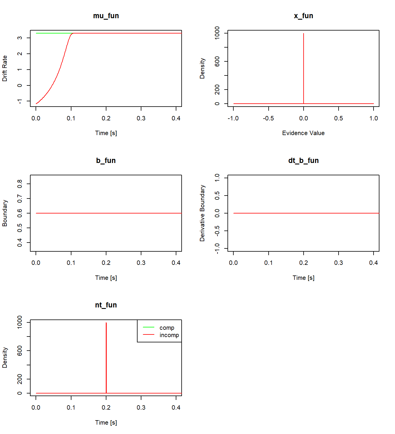
Figure 5.5: A visualization of all evaluated component functions for the re-implemented SSP model.

5.2.2 Collapsing Boundaries and a Custom starting Point

As a second example, we demonstrate how to implement a collapsing boundary and a custom starting point distribution.³³ The collapsing boundary we implement follows a hyperbolic ratio function proposed by Voskuilen, Ratcliff, and Smith (2016). The upper threshold is defined as

\[ b(t) = b_0 \left(1 - \kappa \cdot \frac{t}{t + t_{0.5}} \right)\,. \]

Here, \(b_0\) is the initial value of the (upper) boundary at \(t=0\) and \(\kappa\) is the proportion of the collapse. For \(\kappa>0\), the function is monotonically decreasing with an asymptote at \(b_0\cdot(1-\kappa)\) for \(t\rightarrow \infty\). \(t_{0.5}\) is the time point at which the boundary has collapsed by half from its initial value to its asymptote. Since dRiftDM assumes symmetric boundaries, the lower bound is given by \(-b(t)\).

To derive a model’s PDFs, we must also provide the derivative of the boundary. For this function, the derivative of \(b(t)\) with respect to \(t\) is

\[ \frac{db(t)}{dt} = -\left(\frac{b_0 \cdot \kappa \cdot t_{0.5}}{(t + t_{0.5})^2} \right)\,. \]

The following functions implement the equations:

# the boundary function
cust_b <- function(prms_model, prms_solve, t_vec, one_cond, ddm_opts) {
  b0 <- prms_model[["b0"]]
  kappa <- prms_model[["kappa"]]
  t05 <- prms_model[["t05"]]

  return(b0 * (1 - kappa * t_vec / (t_vec + t05)))
}

# the derivative of the boundary function
cust_dt_b <- function(prms_model, prms_solve, t_vec, one_cond, ddm_opts) {
  b0 <- prms_model[["b0"]]
  kappa <- prms_model[["kappa"]]
  t05 <- prms_model[["t05"]]

  return(-(b0 * kappa * t05) / (t_vec + t05)^2)
}

Next, we define a function that describes the starting point distribution. For demonstration purposes, we use a symmetric beta-shaped distribution. Since dRiftDM normalizes the evidence space to the interval \([-1, 1]\), but the beta distribution is defined over \([0, 1]\), we must rescale the input before evaluating the beta PDF. Specifically, the rescaled starting point density is:

\[ x_0(x) = f\left(\frac{x}{2} + 0.5;\, \alpha, \alpha \right) \quad \text{for} \quad x \in [-1, 1] \]

Here, \(f\) denotes the PDF of the beta distribution, and \(\alpha\) is a shape parameter. The following code chunk defines a corresponding function:

cust_x <- function(prms_model, prms_solve, x_vec, one_cond, ddm_opts) {
  alpha <- prms_model[["alpha"]]
  dx <- prms_solve[["dx"]]
  start_dist <- dbeta(x_vec / 2 + 0.5, alpha, alpha)
  # ensure that it "integrates" to 1 and pass back
  start_dist <- start_dist / (sum(start_dist) * dx)
  return(start_dist)
}

There are two important considerations when defining this function. First, dRiftDM requires that any function passed to x_fun accepts an argument x_vec, which represents the discretized evidence space. Second, dRiftDM includes internal checks to ensure that the output of x_fun roughly integrates to 1. This prevents users from accidentally supplying a function that does not define a valid PDF.

The last step is to write again a function that assembles our custom model by calling drift_dm():

my_cust_model <- function() {
  # define parameters and conditions
  # b0, kappa, and t05 are required by our custom boundary functions
  # alpha is required by our custom starting point distribution
  # muc is required by the constant drift rate
  # non_dec is required for the non-decision time
  prms_model <- c(
    b0 = 0.6, kappa = 0.5, t05 = 0.15, alpha = 3,
    muc = 4, non_dec = 0.3
  )
  conds <- c("null") # only one condition... we label it null

  # provides access to pre-build component functions
  comps <- component_shelf()

  # call the drift_dm function which is the backbone of dRiftDM
  dm <- drift_dm(
    prms_model = prms_model,
    conds = conds,
    subclass = "coll_start_dm",
    mu_fun = comps$mu_constant,          # constant drift rate with parameter muc
    mu_int_fun = comps$mu_int_constant,  # integral of drift rate
    x_fun = cust_x,                      # custom beta-shaped start distribution
    b_fun = cust_b,                      # custom collapsing boundary
    dt_b_fun = cust_dt_b,                # derivative of custom boundary
    nt_fun = comps$nt_constant           # const. non-decision time named non_dec
  )

  return(dm)
}

The parameters b0, kappa, t05, and alpha are those required by our custom boundary and starting point functions. The remaining parameters muc and non_dec are those required for the constant drift rate and non-decision time (see also the documentation of component_shelf()). Figure 5.6 shows a plot of the evaluated component functions of the model.

cust_model <- my_cust_model()
plot(cust_model)

Figure 5.6: A visualization of all evaluated component functions for a model with custom boundaries and starting point distribution.

5.3 Exercise: Write Your Own Model

Design a DDM that incorporates a custom drift rate, starting point, boundary, or non-decision time, and implement it using dRiftDM. The model does not need to be practically useful, feel free to experiment with any idea that interests you.

If you’re unsure where to start, here are a few suggestions:

Urgency-Modulated Drift Rate: Some DDMs incorporate an urgency signal that scales the incoming information to speed up processing over time. For example, following Hawkins et al. (2015) and Ditterich (2006), this urgency signal \(\gamma(t)\) can be modeled using a three-parameter logistic function:

\[ \gamma(t) = \frac{s_y \cdot e^{s_x \cdot (t - d)}}{1 + e^{s_x \cdot (t - d)}} + \frac{1 + (1 - s_y) \cdot e^{-s_x \cdot d}}{1 + e^{-s_x \cdot d}} \] Here, \(d\) controls the delay (in time units), while \(s_x\) and \(s_y\) shape the curve. A larger \(s_x\) causes a sharper switch from low to high urgency, and a larger \(s_y\) increases the final urgency gain. The resulting time-dependent drift rate is:

\[ \mu(t) = \mu \cdot \gamma(t) \]

where \(\mu\) represents the information quality (as in the classic Ratcliff DDM).³⁴
Reversing Drift Direction: In decision-making research, some models propose that the accumulation of evidence can switch direction during the decision process (Diederich and Oswald 2014). For instance, an evidence accumulation process might initially favor one alternative, but then flips to favor the other at time \(t_{flip}\). Implement a drift rate function where evidence first linearly decreases toward the lower boundary and then reverses toward the upper boundary after \(t_{flip}\).³⁵
Re-implement an Existing Component: Explore the component_shelf() documentation and re-implement one of the existing component functions. For example, re-implement a normally distributed non-decision time, and use it to build a custom version of the Ratcliff DDM.³⁶

5.4 Solution for the Exercise

Because this exercise focused on writing a custom model, there is no single “correct” solution. However, we provide example code below that implements the suggestions outlined above.

Urgency-Modulated Drift Rate:

# custom drift rate with an urgancy signal
mu_urgancy <- function(prms_model, prms_solve, t_vec, one_cond, ddm_opts) {
  # extract all parameters (one row of the parameter matrix)
  s_y <- prms_model[["s_y"]]
  s_x <- prms_model[["s_x"]]
  d <- prms_model[["d"]]
  mu <- prms_model[["mu"]]

  # calculate the urgancy signal
  term1 <- (s_y * exp(s_x * (t_vec - d))) / (1 + exp(s_x * (t_vec - d)))
  term2 <- (1 + (1 - s_y) * exp(-s_x * d)) / (1 + exp(-s_x * d))
  gamma_t <- term1 + term2

  # calculate the drift rate
  mu <- mu * gamma_t
  return(mu)
}

# assembling function
cust_model <- function() {
  # define all parameters and conditions
  prms_model <- c(
    s_y = 8, s_x = 20, d = 0.05, mu = 1, # parameters for the custom drift rate
    b = .6, # parameter for a time-independent boundary "b"
    non_dec = .2 # parameter for a non-decision time "non_dec"
  )
  conds <- c("null") # just one condition

  # get access to pre-built component functions
  comps <- component_shelf()

  # call the drift_dm function
  ddm <- drift_dm(
    prms_model = prms_model,
    conds = conds,
    subclass = "my_custom_model",
    mu_fun = mu_urgancy, # the custom drift rate function
    mu_int_fun = comps$dummy_t, # no integral needed
    x_fun = comps$x_dirac_0, # pre-built dirac delta on zero for the starting point
    b_fun = comps$b_constant, # pre-built time-independent boundary with parameter b
    dt_b_fun = comps$dt_b_constant, # pre-built derivative of the boundary
    nt_fun = comps$nt_constant # pre-built non-decision time with parameter non_dec
  )

  return(ddm)
}

cust_ddm <- cust_model()
plot(
  simulate_traces(cust_ddm, k = 1, sigma = 0),
  xlim = c(0, 0.4)
)

Flipping the Drift Rate:

# custom drift rate with flip
mu_flip <- function(prms_model, prms_solve, t_vec, one_cond, ddm_opts) {
  # extract all parameters (one row of the parameter matrix)
  mu <- prms_model[["mu"]]
  t_flip <- prms_model[["t_flip"]]

  # calculate the drift rate and flip after t_flip
  mu_vec <- rep(-mu, length.out = length(t_vec))
  mu_vec[t_vec > t_flip] <- mu

  return(mu_vec)
}

# assembling function
cust_model <- function() {
  # define all parameters and conditions
  prms_model <- c(
    mu = 3, t_flip = 0.1, # parameters for the custom drift rate
    b = .6, # parameter for a time-independent boundary "b"
    non_dec = .2 # parameter for a non-decision time "non_dec"
  )
  conds <- c("null") # just one condition

  # get access to pre-built component functions
  comps <- component_shelf()

  # call the drift_dm function
  ddm <- drift_dm(
    prms_model = prms_model,
    conds = conds,
    subclass = "my_custom_model",
    mu_fun = mu_flip, # the custom drift rate function
    mu_int_fun = comps$dummy_t, # no integral needed
    x_fun = comps$x_dirac_0, # pre-built dirac delta on zero for the starting point
    b_fun = comps$b_constant, # pre-built time-independent boundary with parameter b
    dt_b_fun = comps$dt_b_constant, # pre-built derivative of the boundary
    nt_fun = comps$nt_constant # pre-built non-decision time with parameter non_dec
  )

  return(ddm)
}

cust_ddm <- cust_model()
plot(
  simulate_traces(cust_ddm, k = 1, sigma = 0),
  xlim = c(0, 0.4)
)

# bonus: change the boundary labels (see the last lines of the summary output)
b_coding(cust_ddm)$column <- "Option"
b_coding(cust_ddm)$u_name_value <- c(A = 1)
b_coding(cust_ddm)$l_name_value <- c(B = 0)
summary(cust_ddm)

## Class(es): my_custom_model, drift_dm
## 
## Current Parameter Matrix:
##      mu t_flip   b non_dec
## null  3    0.1 0.6     0.2
## 
## Unique Parameters:
##      mu t_flip b non_dec
## null  1      2 3       4
## 
## Observed Data:
## NULL
## 
## Fit Indices:
## NULL
## 
## -------
## Deriving PDFs:
##   solver: kfe
##   values: sigma=1, t_max=3, dt=0.001, dx=0.001, nt=3000, nx=2000 
## 
## Boundary Coding:
##   upper: A 
##   lower: B 
##   expected data column: Option (A = 1; B = 0)

A custom Ratcliff DDM, with a normally-distributed non-decision time:

# custom non-decision function (results must be a valid PDF)
cust_nt <- function(prms_model, prms_solve, t_vec, one_cond, ddm_opts) {
  # get the relevant parameters
  non_dec <- prms_model[["non_dec"]]
  sd_non_dec <- prms_model[["sd_non_dec"]]

  # get the settings for the time space discretization
  t_max <- prms_solve[["t_max"]]
  dt <- prms_solve[["dt"]]

  # calculate the density
  d_nt <- dnorm(x = t_vec, mean = non_dec, sd = sd_non_dec)
  d_nt <- d_nt / (sum(d_nt) * dt) # ensure it always "integrates" to 1
  return(d_nt)
}

# assembling function
cust_model <- function() {
  # define all parameters and conditions
  prms_model <- c(
    muc = 3, # parameters for a time-independent drift rate
    b = .6, # parameter for a time-independent boundary "b"
    non_dec = .2, sd_non_dec = .02 # parameter for the custom non-decision time
  )
  conds <- c("null") # just one condition

  # get access to pre-built component functions
  comps <- component_shelf()

  # call the drift_dm function
  ddm <- drift_dm(
    prms_model = prms_model,
    conds = conds,
    subclass = "my_custom_model",
    mu_fun = comps$mu_constant, # pre-built drift rate with parameter muc
    mu_int_fun = comps$mu_int_constant, # corresponding integral of the drift rate
    x_fun = comps$x_dirac_0, # pre-built dirac delta on zero for the starting point
    b_fun = comps$b_constant, # pre-built boundary with parameter b
    dt_b_fun = comps$dt_b_constant, # pre-built derivative of the boundary
    nt_fun = cust_nt # custom non-decision time
  )

  return(ddm)
}

cust_ddm <- cust_model()
plot(cust_ddm)

By default, dRiftDM assigns unique parameter labels and only appends condition-specific labels if a parameter can differ across conditions (excluding special dependencies). This is why, in the following output, the labels “.comp” and “.incomp” appear only for muc, and not for any other parameter.↩︎
This dummy function includes the required arguments but throws an error when called. This ensures that internal checks pass, while any unintended call to the function still triggers an error.↩︎
All of the following functions are already available via component_shelf(), but are re-implemented here for demonstration purposes.↩︎
Default values could be: \(d = 0.05\), \(s_y = 8\), \(s_x = 20\), \(\mu = 1\)↩︎
Bonus: Use b_coding() to relabel decision boundaries from “correct”/“incorrect” to “A”/“B”—see the documentation for details.↩︎
For guidance, see Example 4 in our vignette.↩︎